Compare Trial Types

The following example shows how to access behavioral and neural data for a given recording session and create plots for different trial types

Make sure that you have the AllenSDK installed in your environment

Imports

import numpy as np
import pandas as pd
import seaborn as sns
import matplotlib.pyplot as plt

%matplotlib notebook
%matplotlib inline

# Import allenSDK and check the version, which should be >2.10.2
import allensdk
allensdk.__version__

'2.15.2'

# import the behavior ophys project cache class from SDK to be able to load the data
from allensdk.brain_observatory.behavior.behavior_project_cache import VisualBehaviorOphysProjectCache

/opt/envs/allensdk/lib/python3.8/site-packages/tqdm/auto.py:21: TqdmWarning: IProgress not found. Please update jupyter and ipywidgets. See https://ipywidgets.readthedocs.io/en/stable/user_install.html
  from .autonotebook import tqdm as notebook_tqdm

Load the cache and get data for one experiment

# Set the path to the dataset
cache_dir = '/root/capsule/data/'

# If you are working with data in the cloud in Code Ocean,
# or if you have already downloaded the full dataset to your local machine,
# you can instantiate a local cache
# cache = VisualBehaviorOphysProjectCache.from_local_cache(cache_dir=cache_dir, use_static_cache=True)

# If you are working with the data locally for the first time, you need to instantiate the cache from S3:
cache = VisualBehaviorOphysProjectCache.from_local_cache(cache_dir=cache_dir, use_static_cache=True)
#cache = VisualBehaviorOphysProjectCache.from_s3_cache(cache_dir=cache_dir)

ophys_experiment_table = cache.get_ophys_experiment_table()

Look at a sample of the experiment table

ophys_experiment_table.sample(5)

	equipment_name	full_genotype	mouse_id	reporter_line	driver_line	sex	age_in_days	cre_line	indicator	session_number	...	ophys_container_id	project_code	imaging_depth	targeted_structure	date_of_acquisition	session_type	experience_level	passive	image_set	file_id
ophys_experiment_id
1039693317	MESO.1	Slc17a7-IRES2-Cre/wt;Camk2a-tTA/wt;Ai93(TITL-G...	513630	Ai93(TITL-GCaMP6f)	[Slc17a7-IRES2-Cre, Camk2a-tTA]	F	203.0	Slc17a7-IRES2-Cre	GCaMP6f	4.0	...	1037672792	VisualBehaviorMultiscope4areasx2d	275	VISl	2020-07-30 10:18:17.791596	OPHYS_4_images_H	Novel 1	False	H	1120142530
915243090	MESO.1	Slc17a7-IRES2-Cre/wt;Camk2a-tTA/wt;Ai93(TITL-G...	453911	Ai93(TITL-GCaMP6f)	[Slc17a7-IRES2-Cre, Camk2a-tTA]	M	173.0	Slc17a7-IRES2-Cre	GCaMP6f	3.0	...	1018027878	VisualBehaviorMultiscope	181	VISp	2019-07-31 08:56:17.109568	OPHYS_3_images_A	Familiar	False	A	1085400502
940354166	CAM2P.3	Slc17a7-IRES2-Cre/wt;Camk2a-tTA/wt;Ai93(TITL-G...	459777	Ai93(TITL-GCaMP6f)	[Slc17a7-IRES2-Cre, Camk2a-tTA]	F	181.0	Slc17a7-IRES2-Cre	GCaMP6f	2.0	...	930022332	VisualBehavior	175	VISp	2019-09-05 15:43:21.000000	OPHYS_2_images_A_passive	Familiar	True	A	940418592
1010092804	MESO.1	Vip-IRES-Cre/wt;Ai148(TIT2L-GC6f-ICL-tTA2)/wt	499478	Ai148(TIT2L-GC6f-ICL-tTA2)	[Vip-IRES-Cre]	F	140.0	Vip-IRES-Cre	GCaMP6f	2.0	...	1018027806	VisualBehaviorMultiscope4areasx2d	267	VISl	2020-02-24 08:41:59.392974	OPHYS_2_images_G_passive	Familiar	True	G	1120142312
924198895	MESO.1	Vip-IRES-Cre/wt;Ai148(TIT2L-GC6f-ICL-tTA2)/wt	453990	Ai148(TIT2L-GC6f-ICL-tTA2)	[Vip-IRES-Cre]	M	187.0	Vip-IRES-Cre	GCaMP6f	6.0	...	1018028188	VisualBehaviorMultiscope	296	VISl	2019-08-14 13:16:12.000000	OPHYS_6_images_B	Novel >1	False	B	1085400908

5 rows × 25 columns

Here are all of the unique session types

np.sort(ophys_experiment_table['session_type'].unique())

array(['OPHYS_1_images_A', 'OPHYS_1_images_B', 'OPHYS_1_images_G',
       'OPHYS_2_images_A_passive', 'OPHYS_2_images_B_passive',
       'OPHYS_2_images_G_passive', 'OPHYS_3_images_A', 'OPHYS_3_images_B',
       'OPHYS_3_images_G', 'OPHYS_4_images_A', 'OPHYS_4_images_B',
       'OPHYS_4_images_H', 'OPHYS_5_images_A_passive',
       'OPHYS_5_images_B_passive', 'OPHYS_5_images_H_passive',
       'OPHYS_6_images_A', 'OPHYS_6_images_B', 'OPHYS_6_images_H'],
      dtype=object)

Select an OPHYS_1_images_A experiment, load the experiment data

experiment_id = ophys_experiment_table.query('session_type == "OPHYS_1_images_A"').sample(random_state=10).index[0]
print('getting experiment data for experiment_id {}'.format(experiment_id))
ophys_experiment = cache.get_behavior_ophys_experiment(experiment_id)

getting experiment data for experiment_id 946476556

/opt/envs/allensdk/lib/python3.8/site-packages/hdmf/spec/namespace.py:531: UserWarning: Ignoring cached namespace 'hdmf-common' version 1.3.0 because version 1.5.1 is already loaded.
  warn("Ignoring cached namespace '%s' version %s because version %s is already loaded."
/opt/envs/allensdk/lib/python3.8/site-packages/hdmf/spec/namespace.py:531: UserWarning: Ignoring cached namespace 'core' version 2.2.5 because version 2.5.0 is already loaded.
  warn("Ignoring cached namespace '%s' version %s because version %s is already loaded."

Look at task performance data

We can see that the d-prime metric, a measure of discrimination performance, peaked at 2.14 during this session, indicating mid-range performance.
(d’ = 0 means no discrimination performance, d’ is infinite for perfect performance, but is limited to about 4.5 this dataset due to trial count limitations).

ophys_experiment.get_performance_metrics()

{'trial_count': 489,
 'go_trial_count': 325,
 'catch_trial_count': 48,
 'hit_trial_count': 11,
 'miss_trial_count': 314,
 'false_alarm_trial_count': 4,
 'correct_reject_trial_count': 44,
 'auto_reward_count': 5,
 'earned_reward_count': 11,
 'total_reward_count': 16,
 'total_reward_volume': 0.10200000000000001,
 'maximum_reward_rate': 3.606067930506664,
 'engaged_trial_count': 82,
 'mean_hit_rate': 0.09107934458687789,
 'mean_hit_rate_uncorrected': 0.09030062323224546,
 'mean_hit_rate_engaged': 0.7413614163614164,
 'mean_false_alarm_rate': 0.1831974556974557,
 'mean_false_alarm_rate_uncorrected': 0.16967797967797968,
 'mean_false_alarm_rate_engaged': 0.6666666666666667,
 'mean_dprime': -0.6280628929364763,
 'mean_dprime_engaged': 0.3837839767679964,
 'max_dprime': 0.967421566101701,
 'max_dprime_engaged': 0.967421566101701}

We can build a trial dataframe that tells us about behavior events on every trial. This can be merged with a rolling performance dataframe, which calculates behavioral performance metrics over a rolling window of 100 trials (excluding aborted trials, or trials where the animal licks prematurely).

trials_df = ophys_experiment.trials.merge(
    ophys_experiment.get_rolling_performance_df().fillna(method='ffill'), # performance data is NaN on aborted trials. Fill forward to populate.
    left_index = True,
    right_index = True
)

trials_df.head()

	start_time	stop_time	lick_times	reward_time	reward_volume	hit	false_alarm	miss	is_change	aborted	...	change_time	response_latency	initial_image_name	change_image_name	reward_rate	hit_rate_raw	hit_rate	false_alarm_rate_raw	false_alarm_rate	rolling_dprime
trials_id
0	305.97088	313.22681	[309.5071, 309.77427, 309.94106, 310.1246, 310...	309.12347	0.005	False	False	False	True	False	...	308.994843	0.512257	im065	im077	NaN	NaN	NaN	NaN	NaN	NaN
1	313.47703	314.66132	[313.59405, 313.77752, 313.96101, 314.14447, 3...	NaN	0.000	False	False	False	False	True	...	NaN	NaN	im077	im077	NaN	NaN	NaN	NaN	NaN	NaN
2	314.97825	316.36271	[315.11169, 315.29514, 315.46196, 315.66213, 3...	NaN	0.000	False	False	False	False	True	...	NaN	NaN	im077	im077	NaN	NaN	NaN	NaN	NaN	NaN
3	316.47944	317.46361	[316.69632, 316.9632, 317.14669, 317.56369]	NaN	0.000	False	False	False	False	True	...	NaN	NaN	im077	im077	NaN	NaN	NaN	NaN	NaN	NaN
4	317.98101	319.91561	[318.28122, 318.49814, 318.69795, 318.86475, 3...	NaN	0.000	False	False	False	False	True	...	NaN	NaN	im077	im077	NaN	NaN	NaN	NaN	NaN	NaN

5 rows × 27 columns

Now we can plot performance over the full experiment duration

fig, ax = plt.subplots(2, 1, figsize = (15,5), sharex=True)

ax[0].plot(trials_df['start_time']/60., trials_df['hit_rate'], color='darkgreen')

ax[0].plot(trials_df['start_time']/60., trials_df['false_alarm_rate'], color='darkred')

ax[0].legend(['rolling hit rate', 'rolling false alarm rate'])

ax[1].plot(trials_df['start_time']/60., trials_df['rolling_dprime'], color='black')

ax[1].set_xlabel('trial start time (minutes)')
ax[0].set_ylabel('response rate')
ax[0].set_title('hit and false alarm rates')
ax[1].set_title("d'")

fig.tight_layout()

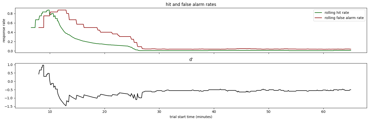
Some key observations:

• The hit rate remains high for the first ~46 minutes of the session

• The false alarm rate graduall declines during the first ~25 minutes of the session.

• d’ peaks when the hit rate is still high, but the false alarm rate dips

• The hit rate and d’ fall off dramatically after ~46 minutes. This is likely due to the animal becoming sated and losing motivation to perform

Plot neural data, behavior, and stimulus information for a trial

Stimulus presentations

Lets look at the dataframe of stimulus presentations. This tells us the attributes of every stimulus that was shown in the session

stimulus_presentations = ophys_experiment.stimulus_presentations
stimulus_presentations.head()

	duration	end_frame	flashes_since_change	image_index	image_name	is_change	omitted	start_frame	start_time	end_time
stimulus_presentations_id
0	0.25022	18001.0	0.0	0	im065	False	False	17986	305.98756	306.23778
1	0.25000	NaN	0.0	8	omitted	False	True	18030	306.72150	306.97150
2	0.25021	18091.0	1.0	0	im065	False	False	18076	307.48881	307.73902
3	0.25019	18136.0	2.0	0	im065	False	False	18121	308.23943	308.48962
4	0.25021	18181.0	0.0	1	im077	True	False	18166	308.99001	309.24022

Note that there is an image name called ‘omitted’. This represents the time that a stimulus would have been shown, had it not been omitted from the regular stimulus cadence. They are included here for ease of analysis, but it’s important to note that they are not actually stimuli. They are the lack of expected stimuli.

stimulus_presentations.query('image_name == "omitted"').head()

	duration	end_frame	flashes_since_change	image_index	image_name	is_change	omitted	start_frame	start_time	end_time
stimulus_presentations_id
1	0.25	NaN	0.0	8	omitted	False	True	18030	306.72150	306.97150
12	0.25	NaN	7.0	8	omitted	False	True	18525	314.97825	315.22825
33	0.25	NaN	1.0	8	omitted	False	True	19470	330.74111	330.99111
42	0.25	NaN	9.0	8	omitted	False	True	19875	337.49660	337.74660
66	0.25	NaN	6.0	8	omitted	False	True	20955	355.51131	355.76131

Running speed

One entry for each read of the analog input line monitoring the encoder voltage, polled at ~60 Hz.

ophys_experiment.running_speed.head()

	timestamps	speed
0	5.97684	0.022645
1	5.99360	2.234085
2	6.01018	4.367226
3	6.02686	6.337823
4	6.04354	8.063498

Licks

One entry for every detected lick onset time, assigned the time of the corresponding visual stimulus frame.

ophys_experiment.licks.head()

	timestamps	frame
0	8.44550	148
1	10.09646	247
2	50.69616	2681
3	50.94637	2696
4	72.69742	4000

Eye tracking data

One entry containing ellipse fit parameters for the eye, pupil and corneal reflection for every frame of the eye tracking video stream.

ophys_experiment.eye_tracking.head()

	timestamps	cr_area	eye_area	pupil_area	likely_blink	pupil_area_raw	cr_area_raw	eye_area_raw	cr_center_x	cr_center_y	...	eye_center_x	eye_center_y	eye_width	eye_height	eye_phi	pupil_center_x	pupil_center_y	pupil_width	pupil_height	pupil_phi
frame
0	0.42068	208.304081	66690.199475	14852.461632	False	14852.461632	208.304081	66690.199475	313.893949	275.783870	...	331.879196	267.942025	162.943138	130.279495	0.055473	331.518456	267.277981	64.946794	68.758166	0.487738
1	0.43153	211.683443	67246.531870	14894.844884	False	14894.844884	211.683443	67246.531870	314.648703	274.890199	...	333.166388	267.938712	162.592435	131.649642	0.049750	332.149275	267.294598	66.021009	68.856201	0.455899
2	0.44081	213.529562	67260.825064	14763.415717	False	14763.415717	213.529562	67260.825064	314.224868	274.586975	...	332.547380	267.146070	162.991558	131.355181	0.038800	331.494585	266.882232	65.201056	68.551741	0.448700
3	0.47454	197.017497	67003.186733	14861.325140	False	14861.325140	197.017497	67003.186733	313.137500	276.562338	...	332.315725	268.699396	162.297228	131.411836	0.043076	330.827633	269.505806	65.011954	68.778679	0.540266
4	0.49075	184.506202	66531.120928	14813.194293	False	14813.194293	184.506202	66531.120928	312.833888	276.887232	...	331.257388	269.569497	162.378660	130.420546	0.042803	330.691566	269.404159	65.289862	68.667213	0.227099

5 rows × 23 columns

Neural data as deltaF/F

One row per cell, with each containing an array of deltaF/F values.

ophys_experiment.dff_traces.head()

	cell_roi_id	dff
cell_specimen_id
1086677732	1080782769	[0.19445239017441418, 0.12601236314041633, 0.1...
1086677737	1080782784	[0.20871294449813774, 0.3277438520090626, 0.14...
1086677746	1080782868	[0.2461564600926237, 0.2061539632478795, 0.183...
1086677771	1080782948	[0.23367534487212552, 0.22006350260557936, 0.2...
1086677774	1080782973	[1.1538649539919354, 0.5792651430717506, 0.386...

We can convert the dff_traces to long-form (aka “tidy”) as follows:

def get_cell_timeseries_dict(dataset, cell_specimen_id):
    '''
    for a given cell_specimen ID, this function creates a dictionary with the following keys
    * timestamps: ophys timestamps
    * cell_roi_id
    * cell_specimen_id
    * dff
    This is useful for generating a tidy dataframe, which can enable easier plotting of timeseries data

    arguments:
        session object
        cell_specimen_id
    returns
        dict
    '''
    cell_dict = {
        'timestamps': dataset.ophys_timestamps,
        'cell_roi_id': [dataset.dff_traces.loc[cell_specimen_id]['cell_roi_id']] * len(dataset.ophys_timestamps),
        'cell_specimen_id': [cell_specimen_id] * len(dataset.ophys_timestamps),
        'dff': dataset.dff_traces.loc[cell_specimen_id]['dff'],

    }
    return cell_dict

ophys_experiment.tidy_dff_traces = pd.concat(
    [pd.DataFrame(get_cell_timeseries_dict(ophys_experiment, cell_specimen_id)) for cell_specimen_id in ophys_experiment.dff_traces.reset_index()['cell_specimen_id']]).reset_index(drop=True)

ophys_experiment.tidy_dff_traces.sample(5)

	timestamps	cell_roi_id	cell_specimen_id	dff
32510917	312.56102	1080792625	1086679879	0.026697
23829986	466.79863	1080789529	1086679311	-0.039413
9230542	4028.75641	1080784412	1086672106	-0.070148
33296257	3055.64495	1080792805	1086679910	0.046809
4094727	1039.20338	1080783601	1086678008	-0.024470

Plot all the data streams for different trial types

We can look at a few trial types in some detail

Define plotting functions

First define functions to plot the different data streams:

each stimulus as a colored vertical bar
running speed
licks/rewards
pupil area
neural responses (dF/F)

def add_image_colors(stimulus_presentations):
    '''
    Add a column to stimulus_presentations called 'color' with a unique color for each image in the session
    '''
    # gather image names but exclude image_name=='omitted'
    unique_stimuli = [stimulus for stimulus in stimulus_presentations['image_name'].unique() if stimulus != 'omitted']
    # assign a color for each unique stimulus
    colormap = {image_name: sns.color_palette()[image_number] for image_number, image_name in enumerate(np.sort(unique_stimuli))}
    colormap['omitted'] = [1, 1, 1] # assign white to omitted
    # add color column to stimulus presentations
    stimulus_presentations['color'] = stimulus_presentations['image_name'].map(lambda image_name: colormap[image_name])
    return stimulus_presentations


def plot_stimuli(trial, ax):
    '''
    plot stimuli as colored bars on specified axis
    '''
    stimuli = ophys_experiment.stimulus_presentations.copy()
    stimuli = add_image_colors(stimuli)
    stimuli = stimuli[(stimuli.end_time >= trial['start_time'].values[0]) & 
                      (stimuli.start_time <= trial['stop_time'].values[0])]
    for idx, stimulus in stimuli.iterrows():
        ax.axvspan(stimulus['start_time'], stimulus['end_time'], color=stimulus['color'], alpha=0.5)
    return ax

        
def plot_running(trial, ax):
    '''
    plot running speed for trial on specified axes
    '''
    trial_running_speed = ophys_experiment.running_speed.copy()
    trial_running_speed = trial_running_speed[(trial_running_speed.timestamps >= trial['start_time'].values[0]) & 
                                              (trial_running_speed.timestamps <= trial['stop_time'].values[0])]
    ax.plot(trial_running_speed['timestamps'], trial_running_speed['speed'], color='black')
    ax.set_title('running speed')
    ax.set_ylabel('speed (cm/s)')
    return ax


def plot_licks(trial, ax):
    '''
    plot licks as black dots on specified axis
    '''
    trial_licks = ophys_experiment.licks.copy()
    trial_licks = trial_licks[(trial_licks.timestamps >= trial['start_time'].values[0]) & 
                              (trial_licks.timestamps <= trial['stop_time'].values[0])]
    ax.plot(trial_licks['timestamps'], np.zeros_like(trial_licks['timestamps']),
            marker = 'o', linestyle = 'none', color='black')
    return ax
    

def plot_rewards(trial, ax):
    '''
    plot rewards as blue diamonds on specified axis
    '''
    trial_rewards = ophys_experiment.rewards.copy()
    trial_rewards = trial_rewards[(trial_rewards.timestamps >= trial['start_time'].values[0]) & 
                                  (trial_rewards.timestamps <= trial['stop_time'].values[0])]
    ax.plot(trial_rewards['timestamps'], np.zeros_like(trial_rewards['timestamps']),
            marker = 'd', linestyle = 'none', color='blue', markersize = 10, alpha = 0.25)
    return ax
    

def plot_pupil(trial, ax):
    '''
    plot pupil area on specified axis
    '''
    trial_eye_tracking = ophys_experiment.eye_tracking.copy()
    trial_eye_tracking = trial_eye_tracking[(trial_eye_tracking.timestamps >= trial['start_time'].values[0]) &
                                            (trial_eye_tracking.timestamps <= trial['stop_time'].values[0])]
    ax.plot(trial_eye_tracking['timestamps'], trial_eye_tracking['pupil_area'], color='black')
    ax.set_title('pupil area')
    ax.set_ylabel('pupil area\n')
    return ax
    

def plot_dff(trial, ax):
    '''
    plot each cell's dff response for a given trial
    '''
    # get the tidy dataframe of dff traces we created earlier
    trial_dff_traces = ophys_experiment.tidy_dff_traces.copy()
    # filter to get this trial
    trial_dff_traces = trial_dff_traces[(trial_dff_traces.timestamps >= trial['start_time'].values[0]) & 
                                        (trial_dff_traces.timestamps <= trial['stop_time'].values[0])]
    # plot each cell
    for cell_specimen_id in ophys_experiment.tidy_dff_traces['cell_specimen_id'].unique():
        ax.plot(trial_dff_traces[trial_dff_traces.cell_specimen_id == cell_specimen_id]['timestamps'],
                trial_dff_traces[trial_dff_traces.cell_specimen_id == cell_specimen_id]['dff'])
        ax.set_title('deltaF/F responses')
        ax.set_ylabel('dF/F')
    return ax
    

def make_trial_plot(trial):
    '''
    combine all plots for a given trial
    '''
    fig, axes = plt.subplots(4, 1, figsize = (15, 8), sharex=True)

    for ax in axes:
        plot_stimuli(trial, ax)

    plot_running(trial, axes[0])

    plot_licks(trial, axes[1])
    plot_rewards(trial, axes[1])

    axes[1].set_title('licks and rewards')
    axes[1].set_yticks([])
    axes[1].legend(['licks','rewards'])

    plot_pupil(trial, axes[2])

    plot_dff(trial, axes[3])

    axes[3].set_xlabel('time in session (seconds)')
    fig.tight_layout()
    return fig, axes

Here is a hit trial

stimulus_presentations.columns

Index(['duration', 'end_frame', 'flashes_since_change', 'image_index',
       'image_name', 'is_change', 'omitted', 'start_frame', 'start_time',
       'end_time'],
      dtype='object')

trials = ophys_experiment.trials.copy()
trial = trials[trials.hit==True].sample()
fig, axes = make_trial_plot(trial)

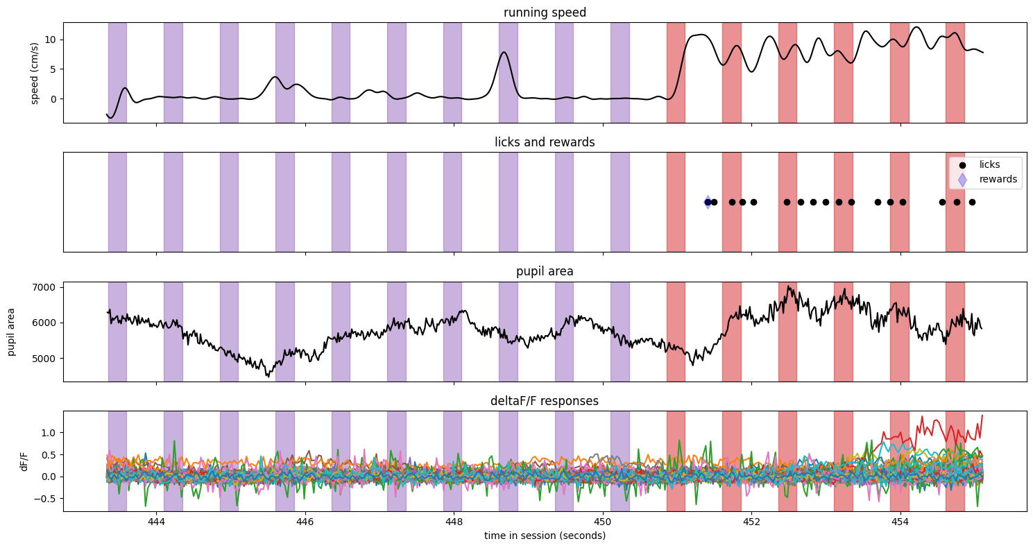
Notes:

• The image identity changed just after t = 2361 seconds (note the color change in the vertical spans)

• The animal was running steadily prior to the image change, then slowed to a stop after the change

• The first lick occured about 500 ms after the change, and triggered an immediate reward

• The pupil area shows some missing data - these were points that were filtered out as outliers.

• There appears to be one neuron that was responding regularly to the stimulus prior to the change.

Here is a miss trial

trial = ophys_experiment.trials.query('miss').sample()
fig, axes = make_trial_plot(trial)

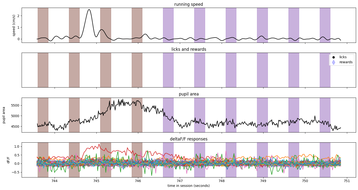
Notes:

• The image identity changed just after t = 824 seconds (note the color change in the vertical spans)

• The animal was running relatively steadily during the entire trial and did not slow after the stimulus identity change

• There were no licks or rewards on this trial

• The pupil area shows some missing data - these were points that were filtered out as outliers.

• One neuron had a large response just prior to the change, but none appear to be stimulus locked on this trial

Here is a false alarm trial

trial = ophys_experiment.trials.query('false_alarm').sample()
fig, axes = make_trial_plot(trial)

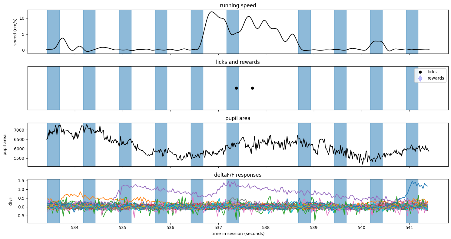
Notes:

• The image identity was consistent during the entire trial

• The animal slowed and licked partway through the trial

• There were no rewards on this trial

• The pupil area shows some missing data - these were points that were filtered out as outliers.

• There were not any neurons with obvious stimulus locked responses

And finally, a correct rejection

trial = ophys_experiment.trials.query('correct_reject').sample()
fig, axes = make_trial_plot(trial)

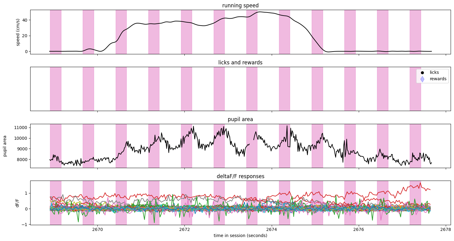
Notes:

• The image identity was consistent during the entire trial

• The animal did not slow or lick during this trial

• There were no rewards on this trial