import numpy as np
import pandas as pd
import matplotlib.pyplot as plt
%matplotlib inline

from allensdk.core.brain_observatory_cache import BrainObservatoryCache
manifest_file = '../../../data/allen-brain-observatory/visual-coding-2p/manifest.json'
boc = BrainObservatoryCache(manifest_file=manifest_file)

Exercise: Evoked response

We want to put these different pieces of data together. Here will will find the preferred image for a neuron - the image among the natural scenes that drives the largest mean response - and see how that response is modulated by the mouse’s running activity.

cell_specimen_id = 517474020
session_id = boc.get_ophys_experiments(cell_specimen_ids=[cell_specimen_id], stimuli=['natural_scenes'])[0]['id']
data_set = boc.get_ophys_experiment_data(ophys_experiment_id=session_id)

Let’s get the cell index for this cell specimen id:

cell_index = data_set.get_cell_specimen_indices([cell_specimen_id])[0]
print("Cell index: ", str(cell_index))

Cell index:  65

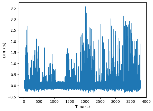
Let’s start with the DF/F traces:

ts, dff = data_set.get_dff_traces()

plt.plot(ts, dff[cell_index,:])
plt.xlabel("Time (s)")
plt.ylabel("DF/F (%)")

Text(0, 0.5, 'DF/F (%)')

Let’s get the stimulus table for the natural scenes:

stim_table = data_set.get_stimulus_table('natural_scenes')
stim_table.head(n=10)

	frame	start	end
0	81	16100	16107
1	33	16108	16115
2	76	16115	16122
3	13	16123	16130
4	56	16130	16137
5	30	16138	16145
6	44	16145	16152
7	93	16153	16160
8	65	16160	16167
9	60	16168	16175

Which image is the preferred image for this neuron?

For each trial of the natural scenes stimulus let’s compute the mean response of the neuron’s response and the mean running speed of the mouse.

num_trials = len(stim_table)

trial_response = np.empty((num_trials))

for index, row in stim_table.iterrows():
    trial_response[index] = dff[cell_index, row.start:row.start+14].mean()

image_response = np.empty((119)) #number of images + blanksweep
image_sem = np.empty((119))
for i in range(-1,118):
    trials = stim_table[stim_table.frame==i].index.values
    image_response[i+1] = trial_response[trials].mean()
    image_sem[i+1] = trial_response[trials].std()/np.sqrt(len(trials))

plt.errorbar(range(-1,118), image_response, yerr=image_sem, fmt='o')
plt.xlabel("Image number")
plt.ylabel("Mean DF/F (%)")

Text(0, 0.5, 'Mean DF/F (%)')

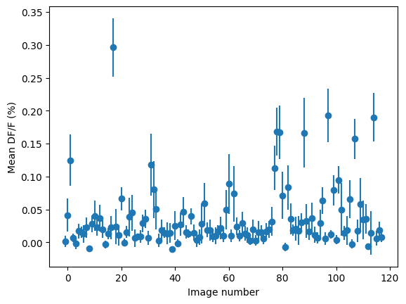
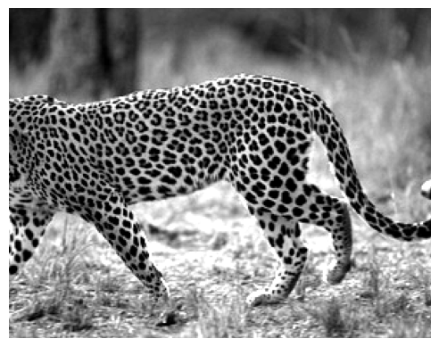
Which image is the preferred image?

preferred_image = np.argmax(image_response) - 1
print(preferred_image)

natural_scene_template = data_set.get_stimulus_template('natural_scenes')
plt.imshow(natural_scene_template[preferred_image,:,:], cmap='gray')
plt.axis('off');

17

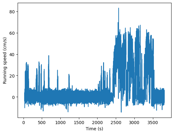
How does the running activity influence the neuron’s response to this image?

Let’s get the running speed of the mouse:

dxcm, _ = data_set.get_running_speed()

plt.plot(ts, dxcm)
plt.xlabel("Time (s)")
plt.ylabel("Running speed (cm/s)")

Text(0, 0.5, 'Running speed (cm/s)')

Compute the mean running speed during each trial. We will make a pandas dataframe with the mean trial response and the mean running speed

trial_speed = np.empty((num_trials))

for index, row in stim_table.iterrows():
    trial_speed[index] = dxcm[row.start:row.end].mean()

df = pd.DataFrame(columns=('response','speed'), index=stim_table.index)
df.response = trial_response
df.speed = trial_speed

stationary_mean = df[(stim_table.frame==preferred_image)&(df.speed<2)].mean()
running_mean = df[(stim_table.frame==preferred_image)&(df.speed>2)].mean()
print("Stationary mean response = ", np.round(stationary_mean.response.mean(),4))
print("Running mean response = ", np.round(running_mean.response.mean(),4))

Stationary mean response =  0.2153
Running mean response =  0.6204

Let’s plot the trial responses when the mouse is stationary (blue) with those when the mouse is running (red).

running_trials = stim_table[(stim_table.frame==preferred_image)&(df.speed>2)].index.values
stationary_trials = stim_table[(stim_table.frame==preferred_image)&(df.speed<2)].index.values

for trial in stationary_trials:
    plt.plot(dff[cell_index, stim_table.start.loc[trial]-30:stim_table.end.loc[trial]+30], color='blue', alpha=0.5)
for trial in running_trials:
    plt.plot(dff[cell_index, stim_table.start.loc[trial]-30:stim_table.end.loc[trial]+30], color='red', alpha=0.5)
plt.axvspan(xmin=30, xmax=37, color='gray', alpha=0.1)
plt.xlabel("Time (frames)")
plt.ylabel("DF/F (%)")

Text(0, 0.5, 'DF/F (%)')

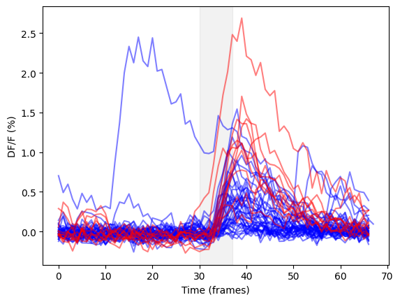
There is a lot of trial-to-trial variability in the response of this neuron to its preferred image. On average, the response during running is larger than that when the mouse is stationary, but there is considerable overlap in the two distributions.