import numpy as np
import pandas as pd
import matplotlib.pyplot as plt
%matplotlib inline

Analysis files and cell specimens table

Analysis file

There are analysis files that accompany each session that contain derived data that might be useful to build upon. However, this should be used with some caution described below.

You can access the analysis object through the BrainObservatoryCache

from allensdk.core.brain_observatory_cache import BrainObservatoryCache
manifest_file = '../../../data/allen-brain-observatory/visual-coding-2p/manifest.json'
boc = BrainObservatoryCache(manifest_file=manifest_file)
experiment_container_id = 511510736
session_id = boc.get_ophys_experiments(experiment_container_ids=[experiment_container_id], stimuli=['natural_scenes'])[0]['id']
data_set = boc.get_ophys_experiment_data(ophys_experiment_id=session_id)

2023-08-21 08:09:27,748 allensdk.api.api.retrieve_file_over_http INFO     Downloading URL: http://api.brain-map.org/api/v2/well_known_file_download/514429113

For each stimulus class there is an analysis function. We demonstrate with Natural Scenes below:

from allensdk.brain_observatory.natural_scenes import NaturalScenes
ns = NaturalScenes(data_set)

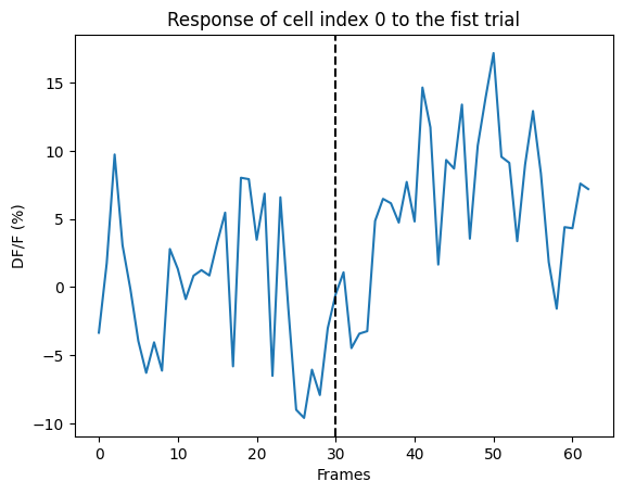
For each stimulus, there are two dataframes called sweep_response and mean_sweep_response that quantify the individual trial responses of each neuron. The sweep_response dataframe contains the DF/F for each neuron for each trial. The index of the dataframe matches the stimulus table for the stimulus, and the columns are the cell indexes (as strings).

For this dataframe, DF/F was computed using the mean fluorescence in the 1 second prior to the start of the trial as the Fo. The sweep response contains this DF/F for each neuron spaning from 1 second before the start of the trial to 1 second after the end of the trial. In addition to the responses of each neuron, there is one additional column that captures the running speed of the mouse during the same time span of each trial. This column is titled ‘dx’.

The mean_sweep_response (with the same index and columns as sweep_response) calculates the mean value of the DF/F in the sweep response dataframe during each trial for each neuron. The column titled ‘dx’ averages the running speed in the same way.

plt.plot(ns.sweep_response['0'].loc[0])
plt.axvline(x=30, ls='--', color='k')
plt.xlabel("Frames")
plt.ylabel("DF/F (%)")
plt.title("Response of cell index 0 to the fist trial")
print("Mean response of cell index 0 to the first trial:", ns.mean_sweep_response['0'].loc[0])

Mean response of cell index 0 to the first trial: 1.9962353

In addition to these dataframes there is a numpy array titled response that captures the mean response to each stimulus condition. For example, for the drifting grating stimulus, this array has the shape of (8,6,3,number_cells+1). The first dimension is the stimulus direction, the second dimension is the temporal frequency plus the blank sweep. The third dimension is [mean response, standard deviation of the response, number of trials of the condition that are significant]. And the last dimension is all the neurons plus the running speed in the last element. So the mean response of, say, cell index 17, to the blank sweep is located at response[0,0,0,17]. For natural scenes this has a shape of (119,3,number_cells+1).

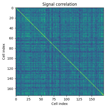
Within this analysis object, there are useful functions to calculate signal and noise correlations called get_signal_correlation and get_noise_correlation. These return arrays of the signal and noise correlations of all the neurons in a session for this specific stimulus. The shape of the array is (number_cells, number_cells).

sc = ns.get_signal_correlation()
plt.imshow(sc[0])
plt.xlabel("Cell index")
plt.ylabel("Cell index")
plt.title("Signal correlation")

Text(0.5, 1.0, 'Signal correlation')

Cell specimen table

In addition the the analysis tables, there are response metrics that have been computed for each neuron using the responses that are stored in the analysis files. These metrics describe the visual activity and response properties of the neurons and can be useful in identifying relevant neurons for analysis. Each metric name has a suffix that is the abbreviation of the stimulus it was computed from (e.g. dg=drifting gratings, lsn=locally sparse noise). These metrics and how they were computed are described extensively in this whitepaper.

cell_specimen_table = pd.DataFrame(boc.get_cell_specimens())
print(cell_specimen_table.keys())
cell_specimen_table.head()

Index(['all_stim', 'area', 'cell_specimen_id', 'donor_full_genotype', 'dsi_dg',
       'experiment_container_id', 'failed_experiment_container', 'g_dsi_dg',
       'g_osi_dg', 'g_osi_sg', 'image_sel_ns', 'imaging_depth', 'osi_dg',
       'osi_sg', 'p_dg', 'p_ns', 'p_run_mod_dg', 'p_run_mod_ns',
       'p_run_mod_sg', 'p_sg', 'peak_dff_dg', 'peak_dff_ns', 'peak_dff_sg',
       'pref_dir_dg', 'pref_image_ns', 'pref_ori_sg', 'pref_phase_sg',
       'pref_sf_sg', 'pref_tf_dg', 'reliability_dg', 'reliability_nm1_a',
       'reliability_nm1_b', 'reliability_nm1_c', 'reliability_nm2',
       'reliability_nm3', 'reliability_ns', 'reliability_sg',
       'rf_area_off_lsn', 'rf_area_on_lsn', 'rf_center_off_x_lsn',
       'rf_center_off_y_lsn', 'rf_center_on_x_lsn', 'rf_center_on_y_lsn',
       'rf_chi2_lsn', 'rf_distance_lsn', 'rf_overlap_index_lsn', 'run_mod_dg',
       'run_mod_ns', 'run_mod_sg', 'sfdi_sg', 'specimen_id', 'tfdi_dg',
       'time_to_peak_ns', 'time_to_peak_sg', 'tld1_id', 'tld1_name', 'tld2_id',
       'tld2_name', 'tlr1_id', 'tlr1_name'],
      dtype='object')

	all_stim	area	cell_specimen_id	donor_full_genotype	dsi_dg	experiment_container_id	failed_experiment_container	g_dsi_dg	g_osi_dg	g_osi_sg	...	specimen_id	tfdi_dg	time_to_peak_ns	time_to_peak_sg	tld1_id	tld1_name	tld2_id	tld2_name	tlr1_id	tlr1_name
0	False	VISp	517397327	Scnn1a-Tg3-Cre/wt;Camk2a-tTA/wt;Ai93(TITL-GCaM...	NaN	511498742	False	NaN	NaN	NaN	...	502185555	NaN	NaN	NaN	177837516	Scnn1a-Tg3-Cre	177837320.0	Camk2a-tTA	265943423	Ai93(TITL-GCaMP6f)
1	False	VISp	517397340	Scnn1a-Tg3-Cre/wt;Camk2a-tTA/wt;Ai93(TITL-GCaM...	1.461268	511498742	False	0.824858	0.901542	NaN	...	502185555	0.333074	NaN	NaN	177837516	Scnn1a-Tg3-Cre	177837320.0	Camk2a-tTA	265943423	Ai93(TITL-GCaMP6f)
2	False	VISp	517397343	Scnn1a-Tg3-Cre/wt;Camk2a-tTA/wt;Ai93(TITL-GCaM...	NaN	511498742	False	0.812462	0.894923	NaN	...	502185555	0.258131	NaN	NaN	177837516	Scnn1a-Tg3-Cre	177837320.0	Camk2a-tTA	265943423	Ai93(TITL-GCaMP6f)
3	False	VISp	517397347	Scnn1a-Tg3-Cre/wt;Camk2a-tTA/wt;Ai93(TITL-GCaM...	NaN	511498742	False	0.078742	0.109241	NaN	...	502185555	0.231590	NaN	NaN	177837516	Scnn1a-Tg3-Cre	177837320.0	Camk2a-tTA	265943423	Ai93(TITL-GCaMP6f)
4	False	VISp	517397353	Scnn1a-Tg3-Cre/wt;Camk2a-tTA/wt;Ai93(TITL-GCaM...	NaN	511498742	False	NaN	NaN	NaN	...	502185555	NaN	NaN	NaN	177837516	Scnn1a-Tg3-Cre	177837320.0	Camk2a-tTA	265943423	Ai93(TITL-GCaMP6f)

5 rows × 60 columns

Caveat

The anaylsis file and the metrics in the cell specimen table were computed from the DF/F as described above. While this is not incorrect, per se, there are some caveats to this. Metrics such as DSI which are defined as (pref-null)/(pref+null) are expected to be contrained to +/- 1. However, we can have trials with negative DF/F, especially using it as we do here, in which case these metrics will not be contrained in this way. This can make it difficult to interpret the resulting values.

These analysis objects and metrics are not invalid, but be sure to use and interpret them appropriately.