import numpy as np
import matplotlib.pyplot as plt
%matplotlib inline

from allensdk.core.brain_observatory_cache import BrainObservatoryCache
manifest_file = '../../../data/allen-brain-observatory/visual-coding-2p/manifest.json'
boc = BrainObservatoryCache(manifest_file=manifest_file)

Getting data from a session

We’re going to examine the data available for a single session. To access the data, we need the experiment session id for the specific session we are interested in. First, let’s identify the session from the experiment container we explored in vc2p-dataset in which that “natural scenes” stimulus was presented.

experiment_container_id = 511510736
session_id = boc.get_ophys_experiments(experiment_container_ids=[experiment_container_id], stimuli=['natural_scenes'])[0]['id']

We can use this session_id to get all the data contained in the NWB for this session using get_ophys_experiment_data

data_set = boc.get_ophys_experiment_data(ophys_experiment_id=session_id)

This data_set object gives us access to a lot of data! Let’s explore:

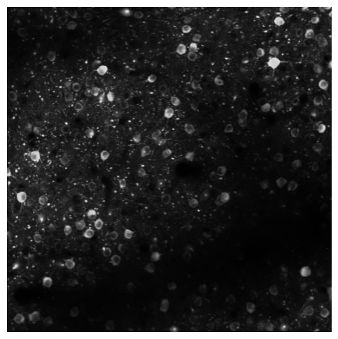
Maximum projection

This is the projection of the full motion corrected movie. It shows all of the cells imaged during the session.

max_projection = data_set.get_max_projection()

fig = plt.figure(figsize=(6,6))
plt.imshow(max_projection, cmap='gray')
plt.axis('off')

(-0.5, 511.5, 511.5, -0.5)

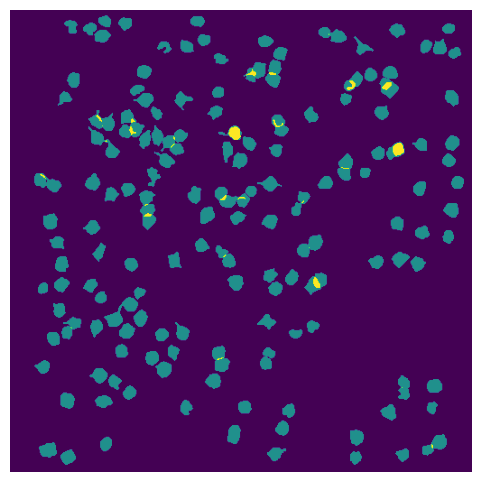
ROI Masks

ROIs are all of the segmented masks for cell bodies identified in this session.

rois = data_set.get_roi_mask_array()

What is the shape of this array? How many neurons are in this experiment?

rois.shape

(174, 512, 512)

The first dimension of this array is the number of neurons, and each element of this axis is the mask of an individual neuron

Plot the masks for all the ROIs.

fig = plt.figure(figsize=(6,6))
plt.imshow(rois.sum(axis=0))
plt.axis('off');

Fluorescence and DF/F traces

The NWB file contains a number of traces reflecting the processing that is done to the extracted fluorescence before we analyze it. The fluorescence traces are the mean fluorescence of all the pixels contained within a ROI mask.

There are a number of activity traces accessible in the NWB file, including raw fluorescence, neuropil corrected traces, demixed traces, and DF/F traces.

timestamps,fluor = data_set.get_fluorescence_traces()

To correct from contamination from the neuropil, we perform neuropil correction. First, we extract a local neuropil signal, by creating a neuropil mask that is an annulus around the ROI mask (without containing any pixels from nearby neurons). You can see these neuropil signals in the neuropil traces:

timestamps, np = data_set.get_neuropil_traces()
r_values = data_set.get_neuropil_r()

This neuropil trace is subtracted from the fluorescence trace, after being weighted by a factor (“r value”) that is computed for each neuron. The resulting corrected fluorescence trace is accessed here along with the r_values.

timestamps,cor = data_set.get_corrected_fluorescence_traces()

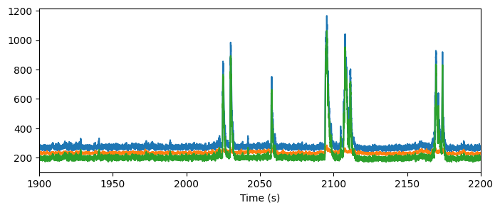
Let’s look at these traces for one cell:

fig = plt.figure(figsize=(8,3))
plt.plot(timestamps, fluor[122,:])
plt.plot(timestamps, np[122,:])
plt.plot(timestamps, cor[122,:])
plt.xlabel("Time (s)")
plt.xlim(1900,2200)

(1900.0, 2200.0)

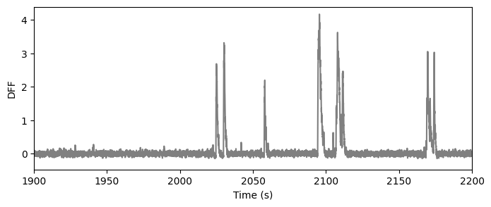
The signal we are most interested in the the DF/F - the change in fluorescence normalized by the baseline fluorescence. The baseline flourescence was computed as the median fluorescence in a 180s window centered on each time point. The result is the dff trace:

ts, dff = data_set.get_dff_traces()

fig = plt.figure(figsize=(8,3))
plt.plot(ts, dff[122,:], color='gray')
plt.xlabel("Time (s)")
plt.xlim(1900,2200)
plt.ylabel("DFF")

Text(0, 0.5, 'DFF')

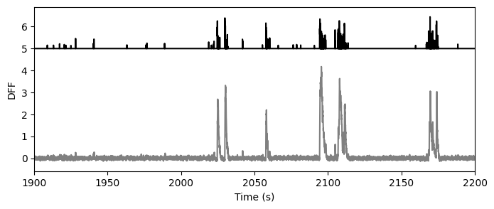
Extracted events

As of the October 2018 data release, we are providing access to events extracted from the DF/F traces using the L0 method developed by Sean Jewell and Daniella Witten.

Note

The extracted events are not stored in the NWB file, thus aren’t a function of the data_set object, but are available through the boc using boc.get_ophys_experiment_events().

events = boc.get_ophys_experiment_events(ophys_experiment_id=session_id)

2023-08-21 08:21:24,438 allensdk.api.api.retrieve_file_over_http INFO     Downloading URL: http://api.brain-map.org/api/v2/well_known_file_download/739721211

fig = plt.figure(figsize=(8,3))
plt.plot(ts, dff[122,:], color='gray')
plt.plot(ts, 2*events[122,:]+5, color='black')
plt.xlabel("Time (s)")
plt.xlim(1900,2200)
plt.ylabel("DFF")

Text(0, 0.5, 'DFF')

Stimulus epochs

Several stimuli are shown during each imaging session, interleaved with each other. The stimulus epoch table provides information of these interleaved stimulus epochs, revealing when each epoch starts and ends. The start and end here are provided in terms of the imaging frame of the two-photon imaging. This allows us to index directly into the dff or event traces.

stim_epoch = data_set.get_stimulus_epoch_table()
stim_epoch

	stimulus	start	end
0	static_gratings	747	15196
1	natural_scenes	16100	30551
2	spontaneous	30701	39581
3	natural_scenes	39582	54050
4	static_gratings	54953	69403
5	natural_movie_one	70307	79338
6	natural_scenes	80241	96126
7	static_gratings	97406	113662

stimulus

The name of the stimulus during the epoch

start

The 2p imaging frame during which the epoch starts. This indexes directly into the activity traces (e.g. dff or extracted events) and behavior traces (e.g. running speed).

end

The 2p imaging frame during which the epoch ends. This indexes directly into the activity traces (e.g. dff or extracted events) and behavior traces (e.g. running speed).

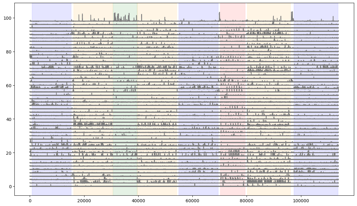
Let’s plot the DFF traces of a number of cells and overlay stimulus epochs.

fig = plt.figure(figsize=(14,8))

#here we plot the first 50 neurons in the session
for i in range(50):
    plt.plot(dff[i,:]+(i*2), color='gray')
    
#here we shade the plot when each stimulus is presented
colors = ['blue','orange','green','red']
for c,stim_name in enumerate(stim_epoch.stimulus.unique()):
    stim = stim_epoch[stim_epoch.stimulus==stim_name]
    for j in range(len(stim)):
        plt.axvspan(xmin=stim.start.iloc[j], xmax=stim.end.iloc[j], color=colors[c], alpha=0.1)

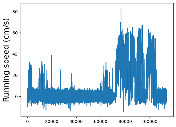
Running speed

The running speed of the animal on the rotating disk during the entire session. This has been temporally aligned to the two photon imaging, which means that this trace has the same length as dff (etc). This also means that the same stimulus start and end information indexes directly into this running speed trace.

dxcm, timestamps = data_set.get_running_speed()
print("length of dff: ", str(len(dff)))
print("length of running speed: ", str(len(dxcm)))

length of dff:  174
length of running speed:  113888

Plot the running speed.

plt.plot(dxcm)
plt.ylabel("Running speed (cm/s)", fontsize=18)

Text(0, 0.5, 'Running speed (cm/s)')

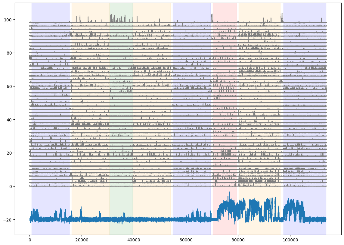
Add the running speed to the neural activity and stimulus epoch figure

fig = plt.figure(figsize=(14,10))
for i in range(50):
    plt.plot(dff[i,:]+(i*2), color='gray')
plt.plot((0.2*dxcm)-20)
    
#for each stimulus, shade the plot when the stimulus is presented
colors = ['blue','orange','green','red']
for c,stim_name in enumerate(stim_epoch.stimulus.unique()):
    stim = stim_epoch[stim_epoch.stimulus==stim_name]
    for j in range(len(stim)):
        plt.axvspan(xmin=stim.start.iloc[j], xmax=stim.end.iloc[j], color=colors[c], alpha=0.1)

Stimulus Table and Template

Each stimulus that is shown has a stimulus table that details what each trial is and when it is presented. Additionally, the natural scenes, natural movies, and locally sparse noise stimuli have a stimulus template that shows the exact image that is presented to the mouse. We detail how to access and use these items in Visual stimuli.

Cell ids and indices

Each neuron in the dataset has a unique id, called the cell specimen id. To find the neurons in this session, get the cell specimen ids. This id can also be used to identify experiment containers or sessions where a given neuron is present

cell_ids = data_set.get_cell_specimen_ids()
cell_ids

array([517473350, 517473341, 517473313, 517473255, 517471959, 517471769,
       517473059, 517471997, 517472716, 517471919, 517472989, 517472293,
       517473115, 517472454, 517473020, 517472734, 517474366, 587377483,
       517471708, 587377366, 587377223, 517474444, 517474437, 517473105,
       517472300, 517472326, 517472708, 517472215, 517472712, 517472360,
       517472399, 517472197, 517472582, 517472190, 517473926, 587377518,
       517471931, 517472637, 517472416, 517471658, 517472724, 517472684,
       517471664, 587377211, 517473947, 587377064, 517472063, 587377621,
       517473080, 517472553, 517473001, 517474078, 517471794, 517471674,
       517473916, 517471803, 517472592, 517473014, 517474459, 517472241,
       517472720, 517472534, 517472054, 587377662, 517474012, 517474020,
       517473653, 517472007, 517472645, 517472211, 517472677, 517472731,
       517472621, 517472442, 587377204, 517473027, 517472818, 517473304,
       517474121, 517473034, 517472909, 517473624, 517472141, 517472129,
       517472903, 517472157, 517474423, 517474430, 517472981, 517472352,
       517471723, 517472116, 517473957, 517472489, 517472123, 517472438,
       517473967, 517474002, 517473991, 517472626, 517473870, 517473374,
       587377633, 517473360, 587377495, 587377673, 517473364, 587377651,
       587377639, 517472470, 517473110, 517473570, 517472897, 517472207,
       517472873, 517471753, 517472563, 517472015, 517472922, 517473980,
       517472135, 517472096, 517472913, 517472524, 517471515, 517472916,
       517473680, 517472162, 517472388, 517474415, 587377657, 587377167,
       517472425, 517472925, 517471912, 587376617, 517472772, 517473098,
       517474342, 517473040, 517473369, 517472807, 587376610, 517473089,
       517472906, 517472462, 587377108, 517472369, 517472900, 517471744,
       517471906, 517472544, 517472503, 517473053, 517472002, 517471785,
       517472919, 517472334, 587377507, 517473897, 517471778, 517472020,
       517472514, 517473067, 587377006, 517471841, 517472180, 517472477,
       587377582, 517473240, 587376723, 517472450, 517473191, 517471925])

Within each individual session, a cell id is associated with an index. This index maps into the dff or event traces. Pick one cell id from the list above and find the index for that neuron.

data_set.get_cell_specimen_indices([517473110])

[110]

Note

As neurons are often matched across sessions, that neuron will have the same cell specimen id in all said sessions, but it will have a different cell specimen index in each session. This is explored in Cross session data.

Session metadata

Each file contains some metadata about that session including fields such as the mouse genotype, sex, and age, the session type, the targeted structure and imaging depth, when the data was acquired, and information about the instrument used to collect the data. This complements metadata used in the boc to identify sessions.

md = data_set.get_metadata()
md

{'sex': 'male',
 'targeted_structure': 'VISp',
 'ophys_experiment_id': 501559087,
 'experiment_container_id': 511510736,
 'excitation_lambda': '910 nanometers',
 'indicator': 'GCaMP6f',
 'fov': '400x400 microns (512 x 512 pixels)',
 'genotype': 'Cux2-CreERT2/wt;Camk2a-tTA/wt;Ai93(TITL-GCaMP6f)/Ai93(TITL-GCaMP6f)',
 'session_start_time': datetime.datetime(2016, 2, 4, 10, 25, 24),
 'session_type': 'three_session_B',
 'specimen_name': 'Cux2-CreERT2;Camk2a-tTA;Ai93-222426',
 'cre_line': 'Cux2-CreERT2/wt',
 'imaging_depth_um': 175,
 'age_days': 104,
 'device': 'Nikon A1R-MP multiphoton microscope',
 'device_name': 'CAM2P.2',
 'pipeline_version': '3.0'}