Units

The primary data in this dataset is the recorded acrtivity of isolated units. A number of metrics are used to isolate units through spike sorting, and these metrics can be used to access how well isolated they are and the quality of each unit. The units dataframe provides many of these metrics, as well as parameterization of the waveform for each unit that passed initial QC, including

• firing rate: mean spike rate during the entire session

• presence ratio: fraction of session when spikes are present

• ISI violations: rate of refractory period violations

• Isolation distances: distance to nearest cluster in Mihalanobis space

• d’: classification accuracy based on LDA

• SNR: signal to noise ratio

• Maximum drift: Maximum change in spike depth during recording

• Cumulative drift: Cumulative change in spike depth during recording

Accessing the units

import os
import numpy as np
import matplotlib.pyplot as plt
%matplotlib inline
import pandas as pd

from allensdk.brain_observatory.ecephys.ecephys_project_cache import EcephysProjectCache

/opt/envs/allensdk/lib/python3.8/site-packages/tqdm/auto.py:21: TqdmWarning: IProgress not found. Please update jupyter and ipywidgets. See https://ipywidgets.readthedocs.io/en/stable/user_install.html
  from .autonotebook import tqdm as notebook_tqdm

# Example cache directory path, it determines where downloaded data will be stored
output_dir = '/root/capsule/data/allen-brain-observatory/visual-coding-neuropixels/ecephys-cache/'
manifest_path = os.path.join(output_dir, "manifest.json")

cache = EcephysProjectCache.from_warehouse(manifest=manifest_path)
session_id = 750332458 # An example session id
session = cache.get_session_data(session_id)

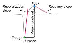
1D Waveform features:

For more information on these:

AllenInstitute/ecephys_spike_sorting AllenInstitute/ecephys_spike_sorting

The units table

The units table contains important information about each unit that was recorded, including its spike sorting quality metrics, its 3D position in the Allen Common Coordinate Framework, and the structure in which it’s located.

Here is a brief summary of the columns in this table:

column name	description
unit_id	the identifier for this unit assigned by the AllenSDK (unique across the entire dataset)
waveform_PT_ratio	peak-to-trough ratio of the average spike waveform
waveform_amplitude	amplitude (in microvolts) of the average spike waveform
amplitude_cutoff	a measure of the approximate fraction of spikes missing from this unit (default threshold = 0.1)
cluster_id	the identifier for this unit assigned by the spike sorting algorithm (unique within each probe)
cumulative_drift	the integrated distance (in microns) that the unit drifted across the whole session
d_prime	a measure of how separable this unit’s waveforms are from its neighbors’
firing_rate	mean spike rate across the whole session
isi_violations	a measure of this unit’s level of contamination (default threshold = 0.5)
isolation_distance	a measure of how separable this unit’s waveforms are from its neighbors’ (higher is better)
L_ratio	a measure of how separable this unit’s waveforms are from its neighbors’ (lower is better)
local_index	the index of this unit within the probe it was recorded with
max_drift	the maximum distance (in microns) the unit drifted across the whole session
nn_hit_rate	a measure of this unit’s level of contamination
nn_miss_rate	a measure of the fraction of spike missing from this unit
peak_channel_id	the identifier for this unit’s peak channel (can be used as an index into the session.channels table
presence_ratio	the fraction of the session over which this unit had spikes detected (default threshold = 0.9)
waveform_recovery_slope	slope of the waveform between the trough and the peak
waveform_repolarization_slope	slope of the waveform back to 0 after the peak
silhouette_score	a measure of this unit’s level of contamination
snr	the ratio of the waveform amplitude relative to the background noise on the peak channel
waveform_spread	distance the waveform extends above and below the peak channel
waveform_velocity_above	speed of waveform propagation above the peak channel
waveform_velocity_below	speed of waveform propagation below the peak channel
waveform_duration	time between the waveform peak and trough
filtering	filter properties of the probe used to record this unit
probe_channel_number	local index of this unit’s peak channel
probe_horizontal_position	horizontal position of this unit on the probe
probe_id	identifier of the probe used to record this unit
probe_vertical_position	vertical position of this unit on the probe
structure_acronym	CCF region where this unit is located
ecephys_structure_id	CCF structure ID where this unit is located
ecephys_structure_acronym	alias for structure_acronym
anterior_posterior_ccf_coordinate	CCF coordinate along the A/P axis
dorsal_ventral_ccf_coordinate	CCF coordinate along the D/V axis
left_right_ccf_coordinate	CCF coordinate along the L/R axis
probe_description	name of the probe used to record this unit
location	not used
probe_sampling_rate	spike band sampling rate of the probe used to record this unit
probe_lfp_sampling_rate	LFP band sampling rate of the probe used to record this unit
probe_has_lfp_data	True if LFP data was recorded on the same probe

Working with the units table

Example: Units

Get the units dataframe for this session.

What the the metrics? (i.e. what are the columns for the dataframe?

How many units are there? How many units per structure?

session.units.head()

	waveform_PT_ratio	waveform_amplitude	amplitude_cutoff	cluster_id	cumulative_drift	d_prime	firing_rate	isi_violations	isolation_distance	L_ratio	...	ecephys_structure_id	ecephys_structure_acronym	anterior_posterior_ccf_coordinate	dorsal_ventral_ccf_coordinate	left_right_ccf_coordinate	probe_description	location	probe_sampling_rate	probe_lfp_sampling_rate	probe_has_lfp_data
unit_id
951817231	0.293351	101.641410	0.001248	8	392.48	6.461795	15.773666	0.020093	147.423046	0.000259	...	8.0	grey	-1000	-1000	-1000	probeA	See electrode locations	29999.968724	1249.998697	True
951817222	1.427508	74.654970	0.032535	7	948.33	5.638511	6.423025	0.007457	95.080849	0.000727	...	8.0	grey	-1000	-1000	-1000	probeA	See electrode locations	29999.968724	1249.998697	True
951817272	0.240866	182.350545	0.000218	13	578.80	4.865528	25.891454	0.002123	121.137882	0.017477	...	8.0	grey	-1000	-1000	-1000	probeA	See electrode locations	29999.968724	1249.998697	True
951817282	0.650177	183.182025	0.000223	14	545.47	4.402664	9.177656	0.001370	59.655811	0.025102	...	8.0	grey	-1000	-1000	-1000	probeA	See electrode locations	29999.968724	1249.998697	True
951817316	0.387017	71.279130	0.059431	18	446.09	3.582546	10.277127	0.050247	56.080395	0.021113	...	8.0	grey	-1000	-1000	-1000	probeA	See electrode locations	29999.968724	1249.998697	True

5 rows × 40 columns

session.units.columns

Index(['waveform_PT_ratio', 'waveform_amplitude', 'amplitude_cutoff',
       'cluster_id', 'cumulative_drift', 'd_prime', 'firing_rate',
       'isi_violations', 'isolation_distance', 'L_ratio', 'local_index',
       'max_drift', 'nn_hit_rate', 'nn_miss_rate', 'peak_channel_id',
       'presence_ratio', 'waveform_recovery_slope',
       'waveform_repolarization_slope', 'silhouette_score', 'snr',
       'waveform_spread', 'waveform_velocity_above', 'waveform_velocity_below',
       'waveform_duration', 'filtering', 'probe_channel_number',
       'probe_horizontal_position', 'probe_id', 'probe_vertical_position',
       'structure_acronym', 'ecephys_structure_id',
       'ecephys_structure_acronym', 'anterior_posterior_ccf_coordinate',
       'dorsal_ventral_ccf_coordinate', 'left_right_ccf_coordinate',
       'probe_description', 'location', 'probe_sampling_rate',
       'probe_lfp_sampling_rate', 'probe_has_lfp_data'],
      dtype='object')

How many units are in this session?

session.units.shape[0]

902

Which areas (structures) are they from?

print(session.units.ecephys_structure_acronym.unique())

['grey' 'VISam' 'VISpm' 'VISp' 'IntG' 'IGL' 'LGd' 'CA3' 'DG' 'CA1' 'VISl'
 'VISal' 'VISrl']

How many units per area are there?

session.units.ecephys_structure_acronym.value_counts()

grey     558
VISal     71
VISp      63
VISam     60
VISrl     44
VISl      38
VISpm     19
CA1       16
CA3       15
DG         7
IGL        5
LGd        4
IntG       2
Name: ecephys_structure_acronym, dtype: int64

Example: Select ‘good’ units

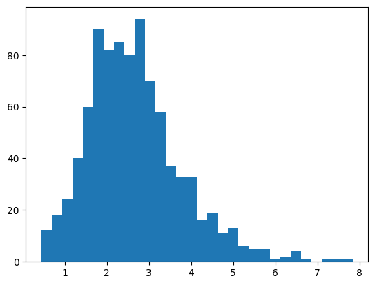
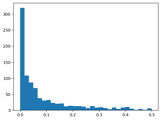
A default is to include units that have a SNR greater than 1 and ISI violations less than 0.5 Plot a histogram of the values for each of these metrics? How many units meet these criteria? How many per structure?

plot a histogram for SNR

plt.hist(session.units.snr, bins=30);

plot a histogram for ISI violations

plt.hist(session.units.isi_violations, bins=30);

good_units = session.units[(session.units.snr>1)&(session.units.isi_violations<0.5)]
len(good_units)

868

good_units.ecephys_structure_acronym.value_counts()

grey     548
VISal     64
VISp      62
VISam     60
VISrl     37
VISl      34
VISpm     18
CA3       15
CA1       15
DG         7
IGL        4
LGd        3
IntG       1
Name: ecephys_structure_acronym, dtype: int64

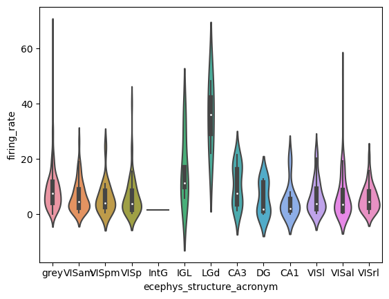
Example: Compare the firing rate of good units in different structures

Make a violinplot of the overall firing rates of units across structures.

import seaborn as sns

sns.violinplot(y='firing_rate', x='ecephys_structure_acronym',data=good_units)

<AxesSubplot:xlabel='ecephys_structure_acronym', ylabel='firing_rate'>

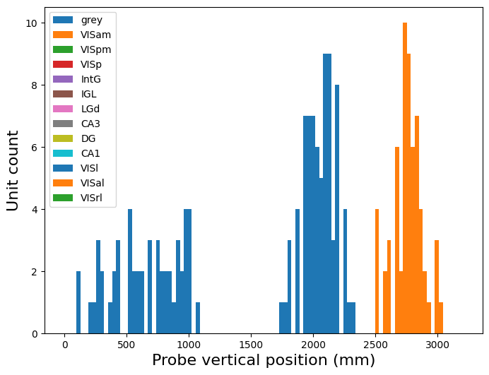
Example: Plot the location of the units on the probe

Color each structure a different color. What do you learn about the vertical position values?

plt.figure(figsize=(8,6))
# restrict to one probe
probe_id = good_units.probe_id.values[0]
probe_units = good_units[good_units.probe_id==probe_id]
for structure in good_units.ecephys_structure_acronym.unique():
    plt.hist(
        probe_units[probe_units.ecephys_structure_acronym==structure].probe_vertical_position.values,
        bins=100, range=(0,3200), label=structure
    )
plt.legend()
plt.xlabel('Probe vertical position (mm)', fontsize=16)
plt.ylabel('Unit count', fontsize=16)
plt.show()

Spike Times

The primary data in this dataset is the recorded acrtivity of isolated units. The spike times is a dictionary of spike times for each units in the session.

Example: Spike Times

Next let’s find the spike_times for these units.

spike_times = session.spike_times

What type of object is this?

type(spike_times)

dict

How many items does it include?

len(spike_times)

902

len(session.units)

902

What are the keys for this object?

list(spike_times.keys())[:5]

[951817566, 951817557, 951818568, 951818561, 951818553]

These keys are unit ids. Use the unit_id for the first unit to get the spike times for that unit. How many spikes does it have in the entire session?

spike_times[session.units.index[0]]

array([3.79596714e+00, 3.81646716e+00, 3.84250052e+00, ...,
       9.75020103e+03, 9.75023709e+03, 9.75027469e+03])

print(len(spike_times[session.units.index[0]]))

153738

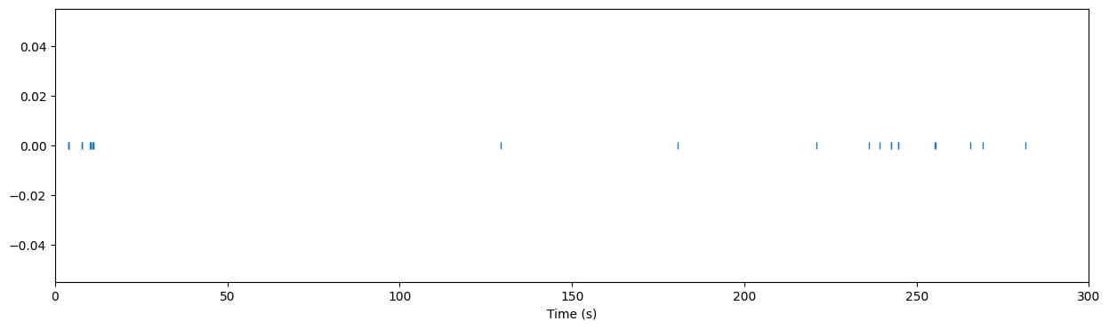
Example: Get the spike times for the units in V1

Use the units dataframe to identify units in ‘VISp’ and use the spike_times to get their spikes. Start just getting the spike times for the first unit identified this way. Plot a raster plot of the spikes during the first 5 minutes (300 seconds) of the experiment.

session.units[session.units.ecephys_structure_acronym=='VISp'].head()

	waveform_PT_ratio	waveform_amplitude	amplitude_cutoff	cluster_id	cumulative_drift	d_prime	firing_rate	isi_violations	isolation_distance	L_ratio	...	ecephys_structure_id	ecephys_structure_acronym	anterior_posterior_ccf_coordinate	dorsal_ventral_ccf_coordinate	left_right_ccf_coordinate	probe_description	location	probe_sampling_rate	probe_lfp_sampling_rate	probe_has_lfp_data
unit_id
951814973	0.599534	26.217945	0.014322	361	345.26	2.927932	1.503416	0.410801	61.132264	0.001457	...	385.0	VISp	-1000	-1000	-1000	probeC	See electrode locations	29999.996461	1249.999853	True
951814989	0.366990	43.292340	0.026720	363	386.49	5.082127	1.885503	0.000000	89.588334	0.001691	...	385.0	VISp	-1000	-1000	-1000	probeC	See electrode locations	29999.996461	1249.999853	True
951816812	0.394103	103.924470	0.002891	561	146.34	4.708563	2.415644	0.046132	80.151626	0.000185	...	385.0	VISp	-1000	-1000	-1000	probeC	See electrode locations	29999.996461	1249.999853	True
951815078	0.329370	111.679035	0.051784	373	165.93	3.799649	4.062188	0.100211	55.356604	0.010204	...	385.0	VISp	-1000	-1000	-1000	probeC	See electrode locations	29999.996461	1249.999853	True
951815150	0.526429	232.830975	0.001259	382	302.18	6.045597	0.516495	0.000000	80.501412	0.000006	...	385.0	VISp	-1000	-1000	-1000	probeC	See electrode locations	29999.996461	1249.999853	True

5 rows × 40 columns

unit_id = session.units[session.units.ecephys_structure_acronym=='VISp'].index[12]

spikes = spike_times[unit_id]
plt.figure(figsize=(15,4))
plt.plot(spikes, np.repeat(0,len(spikes)), '|')
plt.xlim(0,300)
plt.xlabel("Time (s)")

Text(0.5, 0, 'Time (s)')

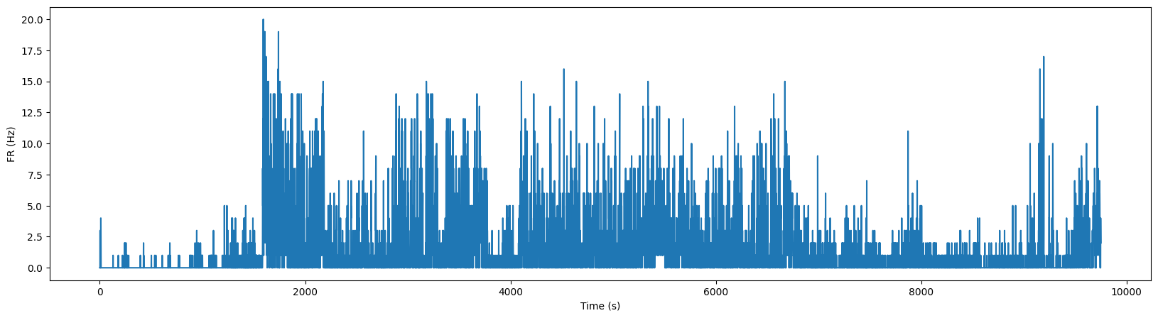
Example: Plot the firing rate for this units across the entire session

A raster plot won’t work for visualizing the activity across the entire session as there are too many spikes! Instead, bin the activity in 1 second bins.

numbins = int(np.ceil(spikes.max()))
binned_spikes = np.empty((numbins))
for i in range(numbins):
    binned_spikes[i] = len(spikes[(spikes>i)&(spikes<i+1)])

plt.figure(figsize=(20,5))
plt.plot(binned_spikes)
plt.xlabel("Time (s)")
plt.ylabel("FR (Hz)")

Text(0, 0.5, 'FR (Hz)')

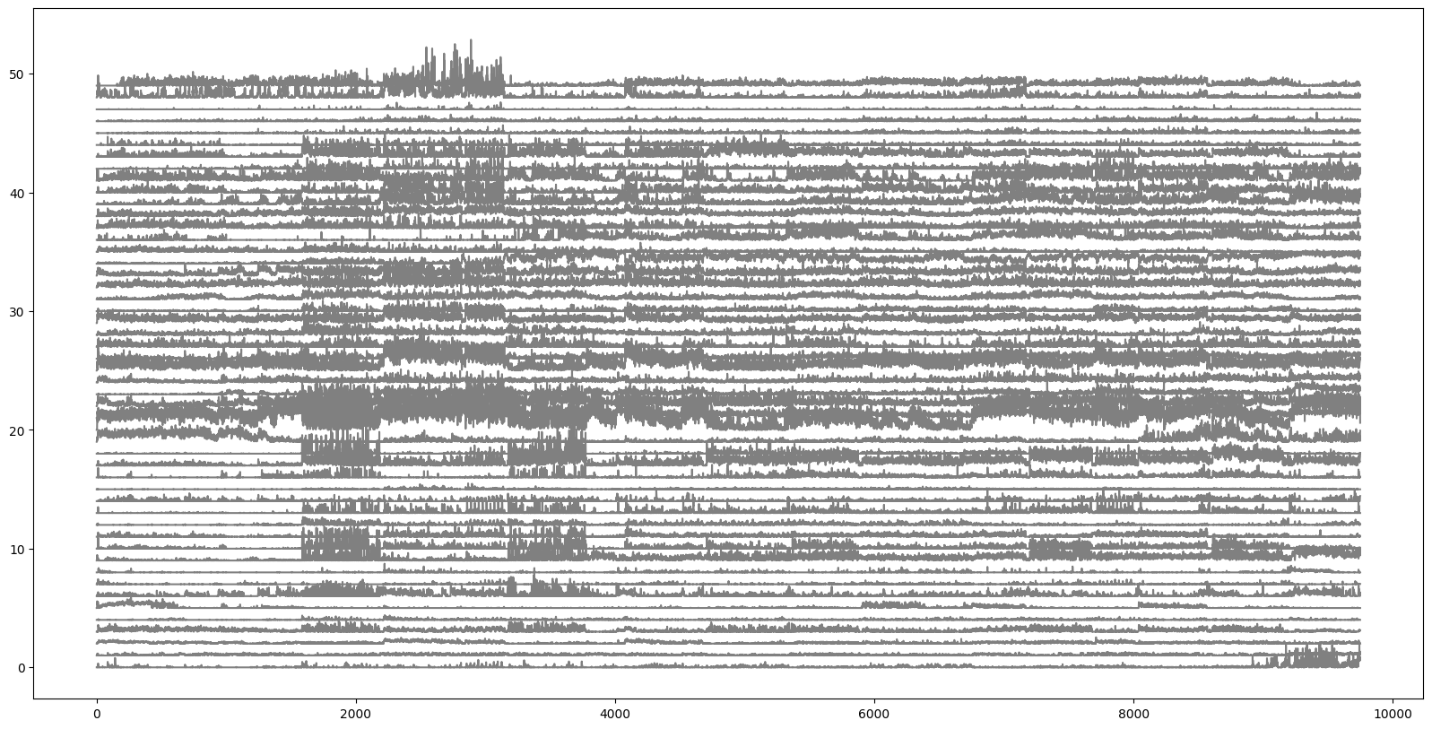
Example: Plot firing rates for units in V1

Now let’s do this for up to 50 units in V1. Make an array of the binned activity of all units in V1 called ‘v1_binned’. We’ll use this again later.

v1_units = session.units[session.units.ecephys_structure_acronym=='VISp']
numunits = len(v1_units)
if numunits>50:
    numunits=50
v1_binned = np.empty((numunits, numbins))
for i in range(numunits):
    unit_id = v1_units.index[i]
    spikes = spike_times[unit_id]
    for j in range(numbins):
        v1_binned[i,j] = len(spikes[(spikes>j)&(spikes<j+1)])

Plot the activity of all the units, one above the other

plt.figure(figsize=(20,10))
for i in range(numunits):
    plt.plot(i+(v1_binned[i,:]/30.), color='gray')

Unit waveforms

For each unit, the average action potential waveform has been recorded from each channel of the probe. This is contained in the mean_waveforms object. This is the characteristic pattern that distinguishes each unit in spike sorting, and it can also help inform us regarding differences between cell types.

We will use this in conjuction with the channel_structure_intervals function which tells us where each channel is located in the brain. This will let us get a feel for the spatial extent of the extracellular action potential waveforms in relation to specific structures.

Example: Unit waveforms

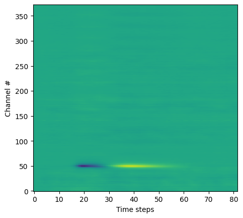
Get the waveform for one unit.

waveforms = session.mean_waveforms

What type of object is this?

type(waveforms)

dict

What are the keys?

list(waveforms.keys())[:5]

[951817566, 951817557, 951818568, 951818561, 951818553]

Get the waveform for one unit

unit = session.units.index.values[400]
wf = session.mean_waveforms[unit]

What type of object is this? What is its shape?

type(wf)

xarray.core.dataarray.DataArray

wf.coords

Coordinates:
  * channel_id  (channel_id) int64 850176026 850176028 ... 850176790 850176792
  * time        (time) float64 0.0 3.333e-05 6.667e-05 ... 0.002667 0.0027

wf.shape

(373, 82)

plt.imshow(wf, aspect=0.2, origin='lower')
plt.xlabel('Time steps')
plt.ylabel('Channel #')

Text(0, 0.5, 'Channel #')

Example: Unit waveforms

Use the channel_structure_intervals to get information about where each channel is located.

We need to pass this function a list of channel ids, and it will identify channels that mark boundaries between identified brain regions.

We can use this information to add some context to our visualization.

# pass in the list of channels from the waveforms data
ecephys_structure_acronyms, intervals = session.channel_structure_intervals(wf.channel_id.values)
print(ecephys_structure_acronyms)
print(intervals)

['grey' 'VISp' nan]
[  0 204 292 373]

Place tick marks at the interval boundaries, and labels at the interval midpoints.

fig, ax = plt.subplots()
plt.imshow(wf, aspect=0.2, origin='lower')
plt.colorbar(ax=ax)

ax.set_xlabel("time (s)")
ax.set_yticks(intervals)
# construct a list of midpoints by averaging adjacent endpoints
interval_midpoints = [ (aa + bb) / 2 for aa, bb in zip(intervals[:-1], intervals[1:])]
ax.set_yticks(interval_midpoints, minor=True)
ax.set_yticklabels(ecephys_structure_acronyms, minor=True)
plt.tick_params("y", which="major", labelleft=False, length=40)

plt.show()

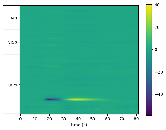
Let’s see if this matches the structure information saved in the units table:

session.units.loc[unit, "ecephys_structure_acronym"]

'grey'

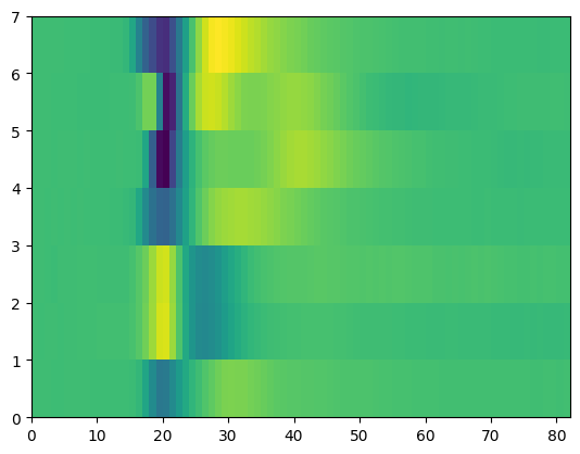
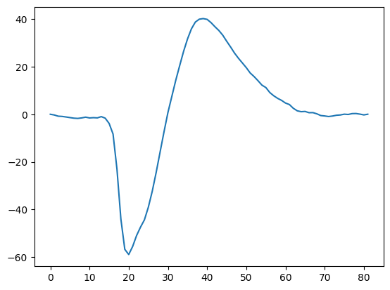
Example: Plot the mean waveform for the peak channel for each unit in the dentate gyrus (DG)

Start by plotting the mean waveform for the peak channel for the unit we just looked at. Then do this for all the units in DG, making a heatmap of these waveforms

Find the peak channel for this unit, and plot the mean waveform for just that channel

channel_id = session.units.loc[unit, 'peak_channel_id']
print(channel_id)

850176126

plt.plot(wf.loc[{"channel_id": channel_id}])

[<matplotlib.lines.Line2D at 0x7fc902f50f40>]

fig, ax = plt.subplots()

th_unit_ids = good_units[good_units.ecephys_structure_acronym=="DG"].index.values

peak_waveforms = []

for unit_id in th_unit_ids:

    peak_ch = good_units.loc[unit_id, "peak_channel_id"]
    unit_mean_waveforms = session.mean_waveforms[unit_id]

    peak_waveforms.append(unit_mean_waveforms.loc[{"channel_id": peak_ch}])


time_domain = unit_mean_waveforms["time"]

peak_waveforms = np.array(peak_waveforms)
plt.pcolormesh(peak_waveforms)

<matplotlib.collections.QuadMesh at 0x7fc9056a42e0>