Receptive fields

Tutorial overview

One of the most important features of visually responsive neurons is the location and extent of their receptive field. Is it highly localized or spatially distributed? Is it centered on the stimulus display, or is it on an edge? How much does it overlap with the receptive fields of neurons in other regions? Obtaining answers to these questions is a crucial step for interpreting a results related to neurons’ visual coding properties.

This Jupyter notebook will cover the following topics:

• Understanding the receptive field stimulus used in the Neuropixels Visual Coding experiments

• Plotting receptive fields for individual units

• Obtaining pre-computed metrics related to receptive fields (coming soon)

• Finding experiments of interest based on receptive field overlap (coming soon)

This tutorial assumes you’ve already created a data cache, or are working with the files on AWS. If you haven’t reached that step yet, we recommend going through the data access tutorial first.

Functions related to additional aspects of data analysis will be covered in other tutorials. For a full list of available tutorials, see the Visual Coding page.

Let’s start by creating an EcephysProjectCache object, and pointing it to a new or existing manifest file:

import os

import numpy as np
import pandas as pd

import matplotlib.pyplot as plt
%matplotlib inline

from allensdk.brain_observatory.ecephys.ecephys_project_cache import EcephysProjectCache

/opt/envs/allensdk/lib/python3.8/site-packages/tqdm/auto.py:21: TqdmWarning: IProgress not found. Please update jupyter and ipywidgets. See https://ipywidgets.readthedocs.io/en/stable/user_install.html
  from .autonotebook import tqdm as notebook_tqdm

If you’re not sure what a manifest file is or where to put it, please check out data access tutorial before going further.

# Example cache directory path, it determines where downloaded data will be stored
output_dir = '/root/capsule/data/allen-brain-observatory/visual-coding-neuropixels/ecephys-cache/'
manifest_path = os.path.join(output_dir, "manifest.json")

cache = EcephysProjectCache.from_warehouse(manifest=manifest_path)

Let’s load the sessions table and grab the data for one experiment in the list:

sessions = cache.get_session_table()
session_id = 759883607 # An example session id
session = cache.get_session_data(session_id)

Finding stimuli in session

In the Visual Coding dataset, a variety of visual stimuli were presented throughout the recording session. The session object contains all of the spike data for one recording session, as well as information about the stimulus, mouse behavior, and probes.

session.stimulus_names

['spontaneous',
 'gabors',
 'flashes',
 'drifting_gratings',
 'natural_movie_three',
 'natural_movie_one',
 'static_gratings',
 'natural_scenes']

Stimulus epochs

These stimuli are interleaved throughout the session. We can use the stimulus_epochs to see when each stimulus type was presented.

stimulus_epochs = session.get_stimulus_epochs()
stimulus_epochs

	start_time	stop_time	duration	stimulus_name	stimulus_block
0	24.737569	84.804349	60.066780	spontaneous	null
1	84.804349	996.849568	912.045219	gabors	0.0
2	996.849568	1285.841049	288.991481	spontaneous	null
3	1285.841049	1584.340430	298.499381	flashes	1.0
4	1584.340430	1586.091909	1.751479	spontaneous	null
5	1586.091909	2185.609422	599.517513	drifting_gratings	2.0
6	2185.609422	2216.635329	31.025907	spontaneous	null
7	2216.635329	2817.137049	600.501720	natural_movie_three	3.0
8	2817.137049	2847.162109	30.025060	spontaneous	null
9	2847.162109	3147.412999	300.250890	natural_movie_one	4.0
10	3147.412999	3177.438049	30.025050	spontaneous	null
11	3177.438049	3776.938972	599.500923	drifting_gratings	5.0
12	3776.938972	4078.190639	301.251667	spontaneous	null
13	4078.190639	4678.692349	600.501710	natural_movie_three	6.0
14	4678.692349	4708.717429	30.025080	spontaneous	null
15	4708.717429	5398.293582	689.576153	drifting_gratings	7.0
16	5398.293582	5399.294419	1.000837	spontaneous	null
17	5399.294419	5879.695809	480.401390	static_gratings	8.0
18	5879.695809	5909.720859	30.025050	spontaneous	null
19	5909.720859	6390.122219	480.401360	natural_scenes	9.0
20	6390.122219	6690.373069	300.250850	spontaneous	null
21	6690.373069	7170.774439	480.401370	natural_scenes	10.0
22	7170.774439	7200.799529	30.025090	spontaneous	null
23	7200.799529	7681.234219	480.434690	static_gratings	11.0
24	7681.234219	7711.259299	30.025080	spontaneous	null
25	7711.259299	8011.510139	300.250840	natural_movie_one	12.0
26	8011.510139	8041.535259	30.025120	spontaneous	null
27	8041.535259	8569.476330	527.941071	natural_scenes	13.0
28	8569.476330	8612.011859	42.535529	spontaneous	null
29	8612.011859	9152.463399	540.451540	static_gratings	14.0

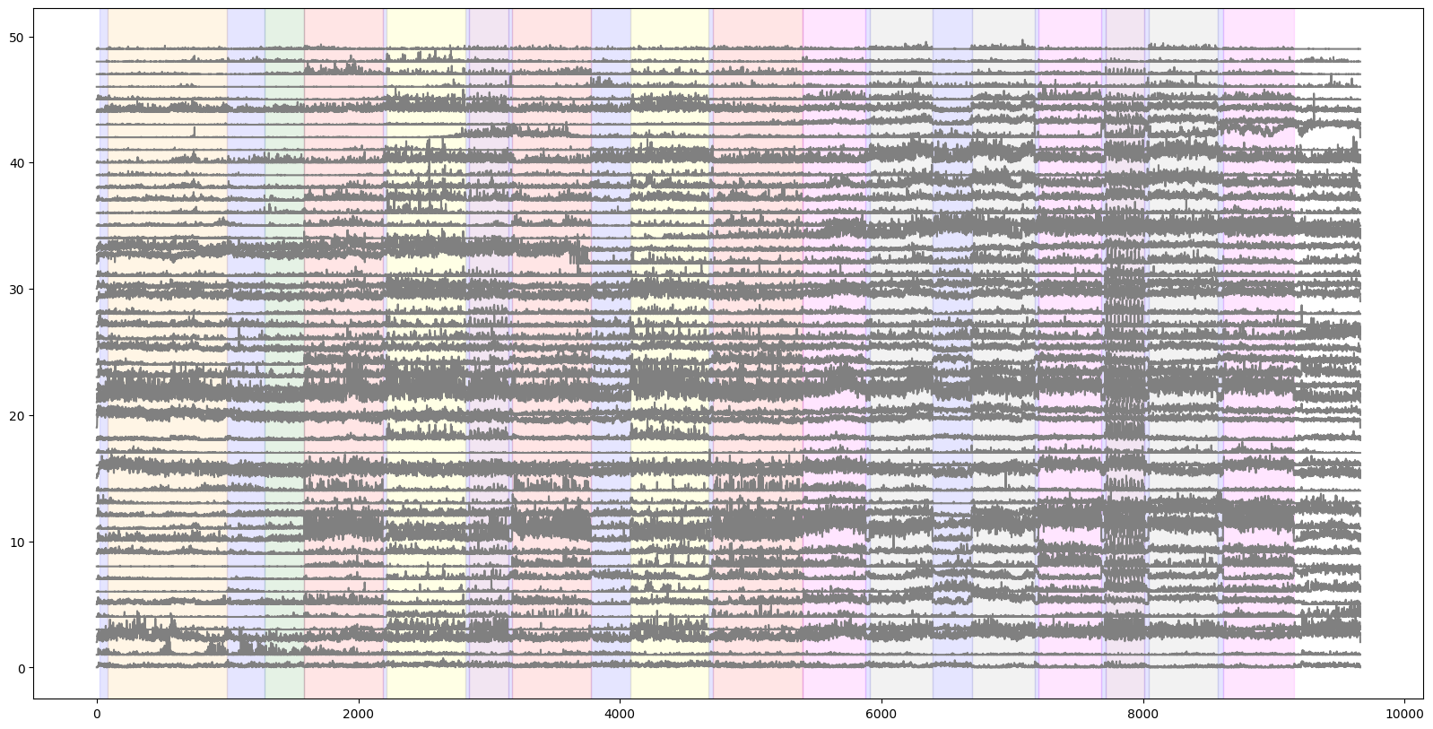
We’ll plot of V1 activity with this stimulus epoch information by shading each stimulus with a unique color. The plt.axvspan() is a useful function for this.

spike_times = session.spike_times
max_spike_time = np.fromiter(map(max, spike_times.values()), dtype=np.double).max()
numbins = int(np.ceil(max_spike_time))
v1_units = session.units[session.units.ecephys_structure_acronym=='VISp']
numunits = min(len(v1_units), 50)
v1_binned = np.empty((numunits, numbins))
for i in range(numunits):
    unit_id = v1_units.index[i]
    spikes = spike_times[unit_id]
    for j in range(numbins):
        v1_binned[i,j] = len(spikes[(spikes>j)&(spikes<j+1)])

plt.figure(figsize=(20,10))
for i in range(numunits):
    plt.plot(i+(v1_binned[i,:]/30.), color='gray')

colors = ['blue','orange','green','red','yellow','purple','magenta','gray','lightblue']
for c, stim_name in enumerate(session.stimulus_names):
    stim = stimulus_epochs[stimulus_epochs.stimulus_name==stim_name]
    for j in range(len(stim)):
        plt.axvspan(xmin=stim["start_time"].iloc[j], xmax=stim["stop_time"].iloc[j], color=colors[c], alpha=0.1)

Running speed

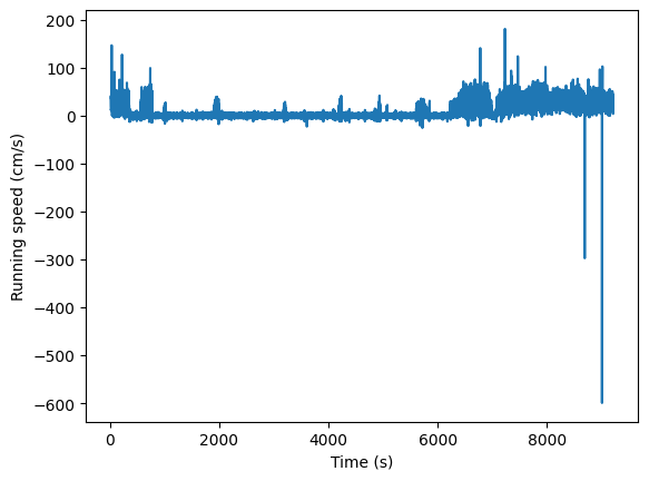
Before we dig further into the stimulus information in more detail, let’s add one more piece of session-wide data to our plot. The mouse’s running speed.

Get the running_speed and its time stamps from the session object. Plot the speed as a function of time.

plt.plot(session.running_speed.end_time, session.running_speed.velocity)
plt.xlabel("Time (s)")
plt.ylabel("Running speed (cm/s)")

Text(0, 0.5, 'Running speed (cm/s)')

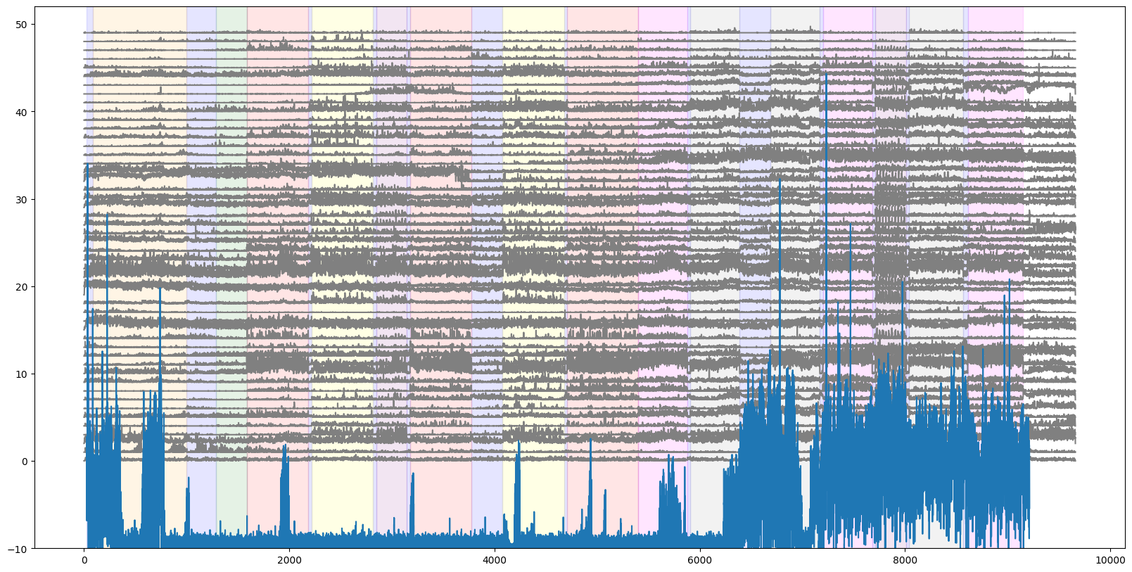
Add the running speed to the plot of V1 activity and stimulus epochs.

plt.figure(figsize=(20,10))
for i in range(numunits):
    plt.plot(i+(v1_binned[i,:]/30.), color='gray')

#scale the running speed and offset it on the plot
plt.plot(session.running_speed.end_time, (0.3*session.running_speed.velocity)-10)

colors = ['blue','orange','green','red','yellow','purple','magenta','gray','lightblue']
for c, stim_name in enumerate(session.stimulus_names):
    stim = stimulus_epochs[stimulus_epochs.stimulus_name==stim_name]
    for j in range(len(stim)):
        plt.axvspan(xmin=stim["start_time"].iloc[j], xmax=stim["stop_time"].iloc[j], color=colors[c], alpha=0.1)

plt.ylim(-10,52)

(-10.0, 52.0)

Stimulus presentations

Now let’s go back and learn more about the stimulus that was presented. The session object has a function that returns a table for a given stimulus called get_stimulus_table.

Use this to get the stimulus table for drifting gratings and for natural scenes.

stim_table = session.get_stimulus_table(['drifting_gratings'])

stim_table.head()

	contrast	orientation	phase	size	spatial_frequency	start_time	stimulus_block	stimulus_name	stop_time	temporal_frequency	duration	stimulus_condition_id
stimulus_presentation_id
3798	0.8	270.0	[5308.98333333, 5308.98333333]	[250.0, 250.0]	0.04	1586.091909	2.0	drifting_gratings	1588.093549	4.0	2.00164	246
3799	0.8	135.0	[5308.98333333, 5308.98333333]	[250.0, 250.0]	0.04	1589.094372	2.0	drifting_gratings	1591.096042	4.0	2.00167	247
3800	0.8	180.0	[5308.98333333, 5308.98333333]	[250.0, 250.0]	0.04	1592.096899	2.0	drifting_gratings	1594.098559	8.0	2.00166	248
3801	0.8	270.0	[5308.98333333, 5308.98333333]	[250.0, 250.0]	0.04	1595.099402	2.0	drifting_gratings	1597.101072	4.0	2.00167	246
3802	0.8	180.0	[5308.98333333, 5308.98333333]	[250.0, 250.0]	0.04	1598.101909	2.0	drifting_gratings	1600.103579	1.0	2.00167	249

Now get the stimulus table for natural scenes.

stim_table_ns = session.get_stimulus_table(['natural_scenes'])

stim_table_ns.head()

	frame	start_time	stimulus_block	stimulus_name	stop_time	duration	stimulus_condition_id
stimulus_presentation_id
51355	92.0	5909.720859	9.0	natural_scenes	5909.971070	0.250211	4908
51356	72.0	5909.971070	9.0	natural_scenes	5910.221280	0.250211	4909
51357	82.0	5910.221280	9.0	natural_scenes	5910.471491	0.250211	4910
51358	55.0	5910.471491	9.0	natural_scenes	5910.721702	0.250211	4911
51359	68.0	5910.721702	9.0	natural_scenes	5910.971898	0.250197	4912

Receptive field mapping stimulus

Because receptive field analysis is so central to interpreting results related to visual coding, every experiment in the Neuropixels Visual Coding dataset includes a standardized receptive field mapping stimulus. This stimulus is always shown at the beginning of the session, and uses the same parameters for every mouse.

We can look at the stimulus_presentations DataFrame in order to examine the parameters of the receptive field mapping stimulus in more detail. The receptive field mapping stimulus consists of drifting Gabor patches with a circular mask, so we’re going to filter the DataFrame based on stimulus_name == 'gabors':

rf_stim_table = session.stimulus_presentations[session.stimulus_presentations.stimulus_name == 'gabors']

len(rf_stim_table)

3645

There are 3645 trials for the receptive field mapping stimulus. What combination of stimulus parameters is used across these trials? Let’s see which parameters actually vary for this stimulus:

keys = rf_stim_table.keys()
[key for key in keys if len(np.unique(rf_stim_table[key])) > 1]

['orientation',
 'start_time',
 'stop_time',
 'x_position',
 'y_position',
 'duration',
 'stimulus_condition_id']

We can ignore the parameters related to stimulus timing (start_time, stop_time, and duration), as well as stimulus_condition_id, which is used to find presentations with the same parameters. So we’re left with orientation, x_position, and y_position.

print('Unique orientations : ' + str(list(np.sort(rf_stim_table.orientation.unique()))))
print('Unique x positions : ' + str(list(np.sort(rf_stim_table.x_position.unique()))))
print('Unique y positions : ' + str(list(np.sort(rf_stim_table.y_position.unique()))))

Unique orientations : [0.0, 45.0, 90.0]
Unique x positions : [-40.0, -30.0, -20.0, -10.0, 0.0, 10.0, 20.0, 30.0, 40.0]
Unique y positions : [-40.0, -30.0, -20.0, -10.0, 0.0, 10.0, 20.0, 30.0, 40.0]

We have 3 orientations and a 9 x 9 grid of spatial locations. Note that these locations are relative to the center of the screen, not the mouse’s center of gaze. How many repeats are there for each condition?

len(rf_stim_table) / (3 * 9 * 9)

15.0

This should match the number we get when dividing the length of the DataFrame by the total number of conditions:

len(rf_stim_table) / len(np.unique(rf_stim_table.stimulus_condition_id))

15.0

What about the drifting grating parameters that don’t vary, such as size (in degrees), spatial frequency (in cycles/degree), temporal frequency (in Hz), and contrast?

print('Spatial frequency: ' + str(rf_stim_table.spatial_frequency.unique()[0]))
print('Temporal frequency: ' + str(rf_stim_table.temporal_frequency.unique()[0]))
print('Size: ' + str(rf_stim_table['size'].unique()[0]))
print('Contrast: ' + str(rf_stim_table['contrast'].unique()[0]))

Spatial frequency: 0.08
Temporal frequency: 4.0
Size: [20.0, 20.0]
Contrast: 0.8

This stimulus is designed to drive neurons reliably across a wide variety of visual areas. Because of the large size (20 degree diameter), it lacks spatial precision. It also cannot be used to map on/off subfields on neurons. However, this is a reasonable compromise to allow us to map receptive fields with high reliability across all visual areas we’re recording from.

Now that we have a better understanding of the stimulus, let’s look at receptive fields for some neurons.

rf_stim_table.keys()

Index(['color', 'contrast', 'frame', 'orientation', 'phase', 'size',
       'spatial_frequency', 'start_time', 'stimulus_block', 'stimulus_name',
       'stop_time', 'temporal_frequency', 'x_position', 'y_position',
       'duration', 'stimulus_condition_id'],
      dtype='object')

Plotting receptive fields

In order to visualize receptive fields, we’re going to use a function in the ReceptiveFieldMapping class, one of the stimulus-specific analysis classes in the AllenSDK. Let’s import it and create a rf_mapping object based on the session we loaded earlier:

from allensdk.brain_observatory.ecephys.stimulus_analysis.receptive_field_mapping import ReceptiveFieldMapping

rf_mapping = ReceptiveFieldMapping(session)

The rf_mapping object contains a variety of methods related to receptive field mapping. Its stim_table property holds the same DataFrame we created earlier.

rf_mapping.stim_table

	contrast	orientation	phase	size	spatial_frequency	start_time	stimulus_block	stimulus_name	stop_time	temporal_frequency	x_position	y_position	duration	stimulus_condition_id
stimulus_presentation_id
1	0.8	0.0	[3644.93333333, 3644.93333333]	[20.0, 20.0]	0.08	84.804349	0.0	gabors	85.037870	4.0	-10.0	-40.0	0.233521	1
2	0.8	0.0	[3644.93333333, 3644.93333333]	[20.0, 20.0]	0.08	85.037870	0.0	gabors	85.288070	4.0	30.0	40.0	0.250201	2
3	0.8	0.0	[3644.93333333, 3644.93333333]	[20.0, 20.0]	0.08	85.288070	0.0	gabors	85.538271	4.0	0.0	0.0	0.250201	3
4	0.8	45.0	[3644.93333333, 3644.93333333]	[20.0, 20.0]	0.08	85.538271	0.0	gabors	85.788472	4.0	-20.0	20.0	0.250201	4
5	0.8	0.0	[3644.93333333, 3644.93333333]	[20.0, 20.0]	0.08	85.788472	0.0	gabors	86.038686	4.0	-40.0	40.0	0.250214	5
...	...	...	...	...	...	...	...	...	...	...	...	...	...	...
3641	0.8	90.0	[3644.93333333, 3644.93333333]	[20.0, 20.0]	0.08	995.598539	0.0	gabors	995.848745	4.0	30.0	-10.0	0.250206	175
3642	0.8	45.0	[3644.93333333, 3644.93333333]	[20.0, 20.0]	0.08	995.848745	0.0	gabors	996.098950	4.0	30.0	10.0	0.250206	228
3643	0.8	0.0	[3644.93333333, 3644.93333333]	[20.0, 20.0]	0.08	996.098950	0.0	gabors	996.349156	4.0	30.0	-20.0	0.250206	156
3644	0.8	90.0	[3644.93333333, 3644.93333333]	[20.0, 20.0]	0.08	996.349156	0.0	gabors	996.599362	4.0	10.0	20.0	0.250206	231
3645	0.8	0.0	[3644.93333333, 3644.93333333]	[20.0, 20.0]	0.08	996.599362	0.0	gabors	996.849568	4.0	-40.0	-30.0	0.250207	72

3645 rows × 14 columns

Before we calculate any receptive fields, let’s find some units in primary visual cortex (VISp) that are likely to show clear receptive fields:

v1_units = session.units[session.units.ecephys_structure_acronym == 'VISp']

Now, calculating the receptive field is as simple as calling get_receptive_field() with a unit ID as the input argument.

RF = rf_mapping.get_receptive_field(v1_units.index.values[3])

This method creates a 2D histogram of spike counts at all 81 possible stimulus locations, and outputs it as a 9 x 9 matrix. It’s summing over all orientations, so each pixel contains the spike count across 45 trials.

To plot it, just display it as an image. The matrix is already in the correct orientation so that it matches the layout of the screen (e.g., the upper right pixel contains the spike count when the Gabor patch was in the upper right of the screen).

plt.figure(figsize=(5,5))
_ = plt.imshow(RF)
_ = plt.axis('off')

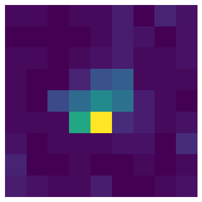
This particular unit has a receptive field that’s more or less in the center of the screen.

Let’s plot the receptive fields for all the units in V1:

def plot_rf(unit_id, index):
    RF = rf_mapping.get_receptive_field(unit_id)
    _ = plt.subplot(6,10,index+1)
    _ = plt.imshow(RF)
    _ = plt.axis('off')

_ = plt.figure(figsize=(10,6))
_ = [plot_rf(RF, index) for index, RF in enumerate(v1_units.index.values)]

Natural scenes stimulus

Use the stimulus table for natural scenes to find all the times when a particular image is presented during the session, and add it to the plot of activity in V1. Pick the first image that was presented in this session.

stim_table_ns[stim_table_ns.frame==stim_table_ns.frame.iloc[0]].head()

	frame	start_time	stimulus_block	stimulus_name	stop_time	duration	stimulus_condition_id
stimulus_presentation_id
51355	92.0	5909.720859	9.0	natural_scenes	5909.971070	0.250211	4908
51494	92.0	5944.499911	9.0	natural_scenes	5944.750122	0.250211	4908
51637	92.0	5980.279805	9.0	natural_scenes	5980.530018	0.250213	4908
51686	92.0	5992.540056	9.0	natural_scenes	5992.790262	0.250206	4908
51735	92.0	6004.800292	9.0	natural_scenes	6005.050501	0.250209	4908

How many times was it presented?

len(stim_table_ns[stim_table_ns.frame==stim_table_ns.frame.iloc[0]])

50

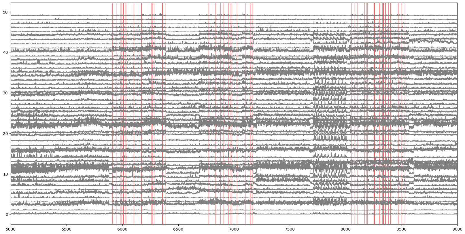
Mark the times when this particular scene was presented on our plot of the activity (without the epochs and running speed).

plt.figure(figsize=(20,10))
for i in range(numunits):
    plt.plot(i+(v1_binned[i,:]/30.), color='gray')

stim_subset = stim_table_ns[stim_table_ns.frame==stim_table_ns.frame.iloc[0]]
for j in range(len(stim_subset)):
    plt.axvspan(xmin=stim_subset.start_time.iloc[j], xmax=stim_subset.stop_time.iloc[j], color='r', alpha=0.5)
plt.xlim(5000,9000)

(5000.0, 9000.0)

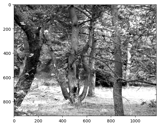
Stimulus template

What is this image? The stimulus template provides the images and movies that were presented to the mouse. These are only provided for stimuli that are images (natural scenes, natural movies) - parametric stimuli (eg. gratings) do not have templates.

image_num = 96
image_template = cache.get_natural_scene_template(image_num)

plt.imshow(image_template, cmap='gray')

<matplotlib.image.AxesImage at 0x7f40d4942b50>

Example: Single trial raster plots for all units

Now that we’ve seen the pieces of data, we can explore the neural activity in greater detail. Make a raster plot for a single presentation of the drifting grating stimulus at orientation = 45 degrees and temporal frequency = 2 Hz.

To start, make a function to make a raster plot of all the units in the experiment.

def plot_raster(spike_times, start, end):
    num_units = len(spike_times)
    ystep = 1 / num_units

    ymin = 0
    ymax = ystep

    for unit_id, unit_spike_times in spike_times.items():
        unit_spike_times = unit_spike_times[np.logical_and(unit_spike_times >= start, unit_spike_times < end)]
        plt.vlines(unit_spike_times, ymin=ymin, ymax=ymax)

        ymin += ystep
        ymax += ystep

Find the first presentation of our chosen grating condition.

stim_table = session.get_stimulus_table(['drifting_gratings'])
subset = stim_table[(stim_table.orientation==45)&(stim_table.temporal_frequency==2)]
start = stim_table.start_time.iloc[0]
end = stim_table.stop_time.iloc[0]

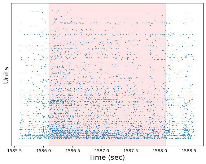
Use the plot_raster function to plot the response of all units to this trial. Pad the raster plot with half a second before and after the trial, and shade the trial red (with an alpha of 0.1)

plt.figure(figsize=(8,6))
plot_raster(session.spike_times, start-0.5, end+0.5)
plt.axvspan(start, end, color='red', alpha=0.1)
plt.xlabel('Time (sec)', fontsize=16)
plt.ylabel('Units', fontsize=16)
plt.tick_params(axis="y", labelleft=False, left=False)
plt.show()

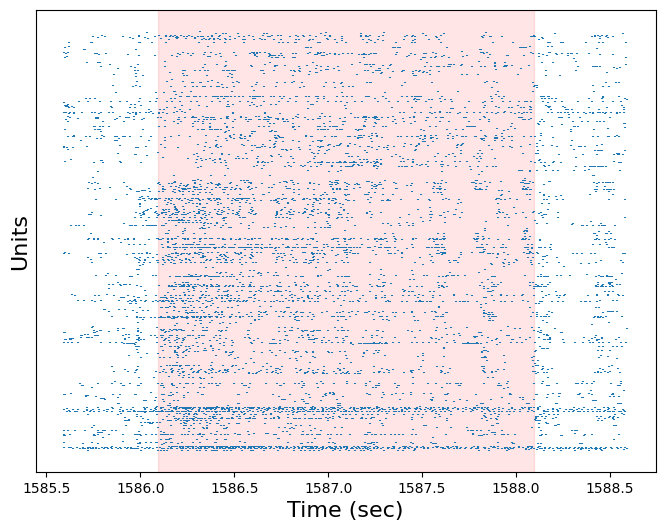
We can use the unit dataframe to arrange the neurons in the raster plot according to their overall firing rate.

session.units.sort_values(by="firing_rate", ascending=False).head()

	waveform_PT_ratio	waveform_amplitude	amplitude_cutoff	cluster_id	cumulative_drift	d_prime	firing_rate	isi_violations	isolation_distance	L_ratio	...	ecephys_structure_id	ecephys_structure_acronym	anterior_posterior_ccf_coordinate	dorsal_ventral_ccf_coordinate	left_right_ccf_coordinate	probe_description	location	probe_sampling_rate	probe_lfp_sampling_rate	probe_has_lfp_data
unit_id
951763835	0.475484	296.48580	0.000030	279	55.08	8.947122	39.043270	0.000051	170.093608	3.380263e-07	...	394.0	VISam	7523	898	7531	probeA	See electrode locations	29999.970168	1249.998757	True
951769847	0.683558	187.32870	0.003021	2	124.35	5.695558	34.004900	0.011311	128.727591	3.679798e-04	...	215.0	APN	7913	3209	7202	probeB	See electrode locations	29999.922149	1249.996756	True
951763130	0.609057	158.42424	0.055363	28	134.27	5.255101	33.830308	0.014039	136.299149	9.153142e-04	...	1061.0	PPT	8205	2618	6750	probeA	See electrode locations	29999.970168	1249.998757	True
951763126	0.738584	260.37843	0.000051	26	121.95	6.741217	31.872133	0.002178	119.811105	2.618902e-04	...	1061.0	PPT	8218	2646	6744	probeA	See electrode locations	29999.970168	1249.998757	True
951763434	0.593540	96.64278	0.000681	176	114.37	3.496612	31.058255	0.007283	124.356326	1.820049e-02	...	382.0	CA1	7719	1438	7110	probeA	See electrode locations	29999.970168	1249.998757	True

5 rows × 40 columns

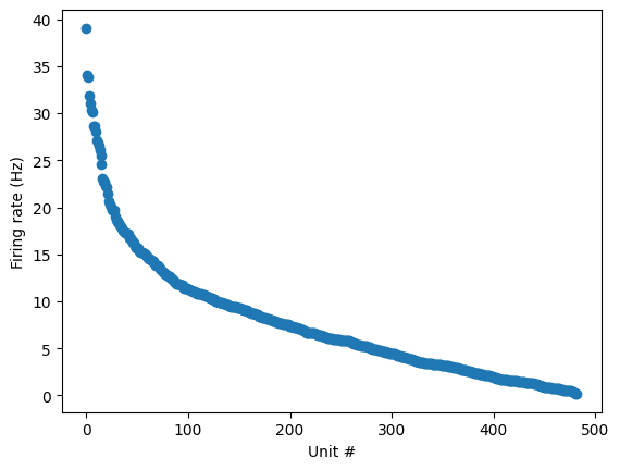
plt.plot(session.units.sort_values(by="firing_rate", ascending=False).firing_rate.values, 'o')
plt.ylabel("Firing rate (Hz)")
plt.xlabel("Unit #")

Text(0.5, 0, 'Unit #')

by_fr = session.units.sort_values(by="firing_rate", ascending=False)
spike_times_by_firing_rate = {
    uid: session.spike_times[uid] for uid in by_fr.index.values
}

plt.figure(figsize=(8,6))
plot_raster(spike_times_by_firing_rate, start-0.5, end+0.5)
plt.axvspan(start, end, color='red', alpha=0.1)
plt.ylabel('Units', fontsize=16)
plt.xlabel('Time (sec)', fontsize=16)
plt.tick_params(axis="y", labelleft=False, left=False)
plt.show()

Stimulus responses

A lot of the analysis of these data will requires comparing responses of neurons to different stimulus conditions and presentations. The SDK has functions to help access these, sorting the spike data into responses for each stimulus presentations and converting from spike times to binned spike counts. This spike histogram representation is more useful for many computations, since it can be treated as a timeseries and directly averaged across presentations.

The presentationwise_spike_counts provides the histograms for specified stimulus presentation trials for specified units. The function requires stimulus_presentation_ids for the stimulus in question, unit_ids for the relevant units, and bin_edges to specify the time bins to count spikes in (relative to stimulus onset).

The conditionwise_spike_statistics creates a summary of specified units responses to specified stimulus conditions, including the mean spike count, standard deviation, and standard error of the mean.

Example: Presentation-wise analysis for drifting gratings

Pick a specific condition of the drifting grating stimulus and create spike histograms for the units in V1. Create bins at a 10 ms resolution so we can see dynamics on a fast timescale.

stim_table.head()

	contrast	orientation	phase	size	spatial_frequency	start_time	stimulus_block	stimulus_name	stop_time	temporal_frequency	duration	stimulus_condition_id
stimulus_presentation_id
3798	0.8	270.0	[5308.98333333, 5308.98333333]	[250.0, 250.0]	0.04	1586.091909	2.0	drifting_gratings	1588.093549	4.0	2.00164	246
3799	0.8	135.0	[5308.98333333, 5308.98333333]	[250.0, 250.0]	0.04	1589.094372	2.0	drifting_gratings	1591.096042	4.0	2.00167	247
3800	0.8	180.0	[5308.98333333, 5308.98333333]	[250.0, 250.0]	0.04	1592.096899	2.0	drifting_gratings	1594.098559	8.0	2.00166	248
3801	0.8	270.0	[5308.98333333, 5308.98333333]	[250.0, 250.0]	0.04	1595.099402	2.0	drifting_gratings	1597.101072	4.0	2.00167	246
3802	0.8	180.0	[5308.98333333, 5308.98333333]	[250.0, 250.0]	0.04	1598.101909	2.0	drifting_gratings	1600.103579	1.0	2.00167	249

# specify the time bins in seconds, relative to stimulus onset
time_step = 1/100.
duration = stim_table.duration.iloc[0]
time_domain = np.arange(0, duration+time_step, time_step)
print(time_domain.shape)

(202,)

stim_ids = stim_table[(stim_table.orientation==90)&(stim_table.temporal_frequency==1)].index
print(stim_ids.shape)

(15,)

histograms = session.presentationwise_spike_counts(bin_edges=time_domain,
                                                   stimulus_presentation_ids=stim_ids,
                                                   unit_ids=v1_units.index)

What type of object is this? What is its shape?

type(histograms)

xarray.core.dataarray.DataArray

histograms.shape

(15, 201, 58)

Xarray

This has returned a new (to this notebook) data structure, the xarray.DataArray. You can think of this as similar to a 3+D pandas.DataFrame, or as a numpy.ndarray with labeled axes and indices. See the xarray documentation for more information. In the mean time, the salient features are:

• Dimensions : Each axis on each data variable is associated with a named dimension. This lets us see unambiguously what the axes of our array mean.

• Coordinates : Arrays of labels for each sample on each dimension.

xarray is nice because it forces code to be explicit about dimensions and coordinates, improving readability and avoiding bugs. However, you can always convert to numpy or pandas data structures as follows:

• to pandas: histograms.to_dataframe() produces a multiindexed dataframe

• to numpy: histograms.values gives you access to the underlying numpy array

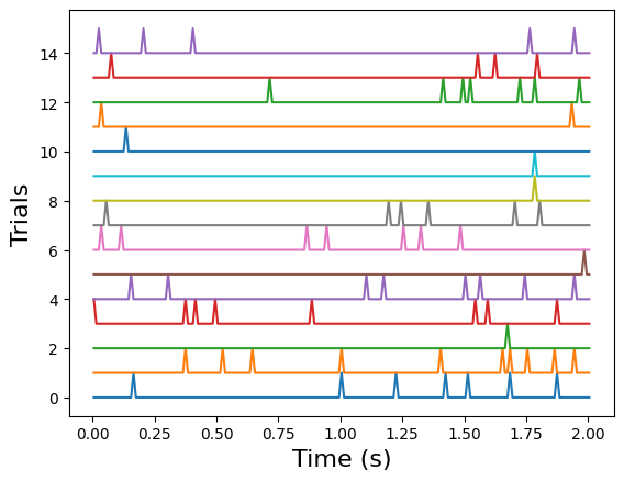
Example: Plot the unit’s response

Plot the response of the first unit to all 15 trials.

for i in range(15):
    plt.plot(histograms.time_relative_to_stimulus_onset, i+histograms[i,:,0])
plt.xlabel("Time (s)", fontsize=16)
plt.ylabel("Trials", fontsize=16)

Text(0, 0.5, 'Trials')

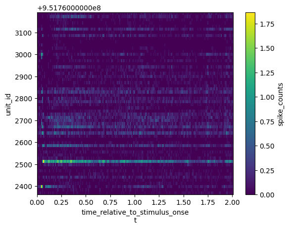
Example: Compute the average response over trials for all units

Plot a heatmap of mean response for all units in V1.

mean_histograms = histograms.mean(dim="stimulus_presentation_id")

mean_histograms.coords

Coordinates:
  * time_relative_to_stimulus_onset  (time_relative_to_stimulus_onset) float64 ...
  * unit_id                          (unit_id) int64 951762582 ... 951762972

import xarray.plot as xrplot
xrplot.imshow(darray=mean_histograms, x="time_relative_to_stimulus_onset",
                                      y="unit_id")

<matplotlib.image.AxesImage at 0x7f40d31c8340>

Example: Conditionwise analysis

In order to compute a tuning curve that summarizes the responses of a unit to each stimulus condition of a stimulus, use the conditionwise_spike_statistics to summarize the activity of specific units to the different stimulus conditions.

stim_ids = stim_table.index.values

dg_stats = session.conditionwise_spike_statistics(stimulus_presentation_ids=stim_ids, unit_ids=v1_units.index)

What type of object is this? What is its shape?

type(dg_stats)

pandas.core.frame.DataFrame

dg_stats.shape

(2378, 5)

What are its columns?

dg_stats.columns

Index(['spike_count', 'stimulus_presentation_count', 'spike_mean', 'spike_std',
       'spike_sem'],
      dtype='object')

Can you explain the first dimension?

dg_stats.head()

		spike_count	stimulus_presentation_count	spike_mean	spike_std	spike_sem
unit_id	stimulus_condition_id
951762582	246	87	15	5.800000	3.967727	1.024463
951762586	246	311	15	20.733333	7.601378	1.962667
951762598	246	65	15	4.333333	5.984106	1.545090
951762602	246	5	15	0.333333	0.617213	0.159364
951762624	246	331	15	22.066667	9.129753	2.357292

Example: Merge the conditionwise statistics with stimulus information

In order to link the stimulus responses with the stimulus conditions, merge the spike_statistics output with the stimulus table using pd.merge().

dg_stats_stim = pd.merge(
    dg_stats.reset_index().set_index(['stimulus_condition_id']),
    session.stimulus_conditions,
    on=['stimulus_condition_id']
).reset_index().set_index(['unit_id', 'stimulus_condition_id'])

This dataframe currently has a multi-index, meaning that each row is indexed by the pair of unit_id and stimulus_condition_id, rather than a single identifier. There are several ways to use this index:

• specify the pair of identifiers as a tuple: dg_stats_stim.loc[(unit_id, stim_id)]

• specifying the axis makes it easier to get all rows for one unit: dg_stats_stim.loc(axis=0)[unit_id, :]

• or you can use dg_stats_stim.reset_index() to move the index to regular columns

dg_stats_stim.head()

		spike_count	stimulus_presentation_count	spike_mean	spike_std	spike_sem	color	contrast	frame	mask	opacity	orientation	phase	size	spatial_frequency	stimulus_name	temporal_frequency	units	x_position	y_position	color_triplet
unit_id	stimulus_condition_id
951762582	246	87	15	5.800000	3.967727	1.024463	null	0.8	null	None	True	270.0	[5308.98333333, 5308.98333333]	[250.0, 250.0]	0.04	drifting_gratings	4.0	deg	null	null	[1.0, 1.0, 1.0]
951762586	246	311	15	20.733333	7.601378	1.962667	null	0.8	null	None	True	270.0	[5308.98333333, 5308.98333333]	[250.0, 250.0]	0.04	drifting_gratings	4.0	deg	null	null	[1.0, 1.0, 1.0]
951762598	246	65	15	4.333333	5.984106	1.545090	null	0.8	null	None	True	270.0	[5308.98333333, 5308.98333333]	[250.0, 250.0]	0.04	drifting_gratings	4.0	deg	null	null	[1.0, 1.0, 1.0]
951762602	246	5	15	0.333333	0.617213	0.159364	null	0.8	null	None	True	270.0	[5308.98333333, 5308.98333333]	[250.0, 250.0]	0.04	drifting_gratings	4.0	deg	null	null	[1.0, 1.0, 1.0]
951762624	246	331	15	22.066667	9.129753	2.357292	null	0.8	null	None	True	270.0	[5308.98333333, 5308.98333333]	[250.0, 250.0]	0.04	drifting_gratings	4.0	deg	null	null	[1.0, 1.0, 1.0]

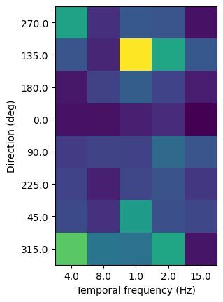
Tuning curve

Let’s plot a 2D tuning curve for the first unit, comparing responses across temporal frequency and orientation.

unit_id = v1_units.index[1]

stim_ids = stim_table.index.values
session.get_stimulus_parameter_values(stimulus_presentation_ids=stim_ids, drop_nulls=True)

{'contrast': array([0.8], dtype=object),
 'orientation': array([270.0, 135.0, 180.0, 0.0, 90.0, 225.0, 45.0, 315.0], dtype=object),
 'phase': array(['[5308.98333333, 5308.98333333]'], dtype=object),
 'size': array(['[250.0, 250.0]'], dtype=object),
 'spatial_frequency': array(['0.04'], dtype=object),
 'temporal_frequency': array([4.0, 8.0, 1.0, 2.0, 15.0], dtype=object)}

orivals = session.get_stimulus_parameter_values(stimulus_presentation_ids=stim_ids, drop_nulls=True)['orientation']
tfvals = session.get_stimulus_parameter_values(stimulus_presentation_ids=stim_ids, drop_nulls=True)['temporal_frequency']

response_mean = np.empty((len(orivals), len(tfvals)))
response_sem = np.empty((len(orivals), len(tfvals)))
for i,ori in enumerate(orivals):
    for j,tf in enumerate(tfvals):
        stim_id = stim_table[(stim_table.orientation==ori)&(stim_table.temporal_frequency==tf)].stimulus_condition_id.iloc[0]
        response_mean[i,j] = dg_stats_stim.loc[(unit_id, stim_id)].spike_mean
        response_sem[i,j] = dg_stats_stim.loc[(unit_id, stim_id)].spike_sem

plt.imshow(response_mean)
plt.xlabel("Temporal frequency (Hz)")
plt.ylabel("Direction (deg)")
plt.xticks(range(5), tfvals)
plt.yticks(range(8), orivals)
plt.show()

Precomputed metrics

This section is not yet complete, but you can use the precomputed metrics provided by the AllenSDK as is described in Precomputed stimulus metrics.