
Meshes#
Important
Before using any programmatic access to the data, you first need to set up your CAVEclient token.
When trying to understand the fine 3d morphology of a neuron (e.g. features under 1 micron in scale), meshes are a particularly useful representation. More precisely, a mesh is a collection of vertices and faces that define a 3d surface. The exact meshes that one sees in Neuroglancer can also be loaded for analysis and visualization in other tools.
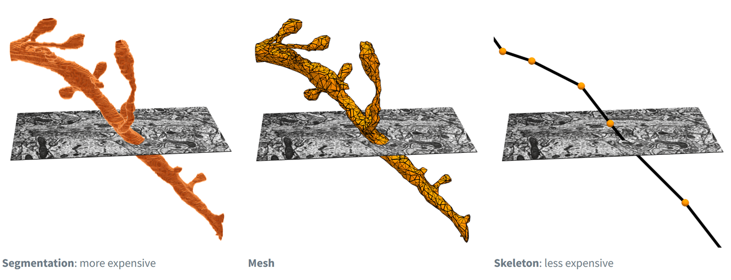
Fig. 50 Electron microscopy data can be represented and rendered in multiple formats, at different levels of abstraction from the original imagery#
Dataset specificity#
The examples below are written with the MICrONS dataset. To access the V1DD dataset change the datastack from minnie65_public to v1dd_public
What is a mesh?#
A mesh is a set of vertices connected via triangular faces to form a 3 dimensional representation of the outer membrane of a neuron, glia or nucleus.
Meshes can either be static or dynamic:#
Static:#
pros: smaller files thus easier to work with, multiple levels of detail (lod) which can be accessed (example below)
cons: may include false gaps and merges from self contacts, updated less frequently
Example path: precomputed://gs://iarpa_microns/minnie/minnie65/seg_m1300
Dynamic:#
pros: highly detailed thus more reflective of biological reality and backed by proofreading infrastructure CAVE (Connectome Annotation Versioning Engine)
cons: much larger files, only one level of detail
Example path: graphene://https://minnie.microns-daf.com/segmentation/table/minnie65_public
Note
At this time the V1DD dataset does not have static meshes. The dynamic meshes can be loaded from the path: graphene://https://api.em.brain.allentech.org/segmentation/table/v1dd_public
Downloading Meshes#
The easiest tool for downloading MICrONs meshes is Meshparty, which is a python module that can be installed with pip install meshparty.
The MeshParty object has more useful properties and attributes such as:
a scipy.csgraph sparse graph object (mesh.csgraph)
a networkx graph object (mesh.nxgraph)
Read more about what you can do with MeshParty on its Documentation.
In particular it lets you associate skeletons, and annotations onto the mesh into a “meshwork” object.
Once installed, the typical way of getting meshes is by using a “MeshMeta” client that is told both the internet location of the meshes (cloud-volume path or cv_path) and a local directory in which to store meshes (disk_cache_path).
Once initialized, the MeshMeta client can be used to download meshes for a given segmentation using its root id (seg_id).
The following code snippet shows how to download an example mesh using a directory “meshes” as the local storage folder.
import os
from meshparty import trimesh_io
from caveclient import CAVEclient
client = CAVEclient('minnie65_public')

# set version, for consistency across time
client.materialize.version = 1507 # Current as of Summer 2025

mm = trimesh_io.MeshMeta(
  cv_path=client.info.segmentation_source(),
  disk_cache_path="meshes",
)

root_id = 864691135545730856
mesh = mm.mesh(seg_id=root_id)
Warning: deduplication not currently supported for this layer's variable layered draco meshes
One convenience of using the MeshMeta approach is that if you have already downloaded a mesh for with a given root id, it will be loaded from disk rather than re-downloaded.
If you have to download many meshes, it is somewhat faster to use the bulk download_meshes function and use multiple threads via the n_threads argument. If you download them to the same folder used for the MeshMeta object, they can be loaded through the same interface.
root_ids = [864691135014128278, 864691135492614239]
mm = trimesh_io.download_meshes(
    seg_ids=root_ids,
    target_dir='meshes',
    cv_path=client.info.segmentation_source(),
    n_threads=4, # Or whatever value you choose above one but less than the number of cores on your computer
)
Note
Meshes can be hundreds of megabytes in size, so be careful about downloading too many if the internet is not acting well or your computer doesn’t have much disk space!
Healing Mesh Gaps#
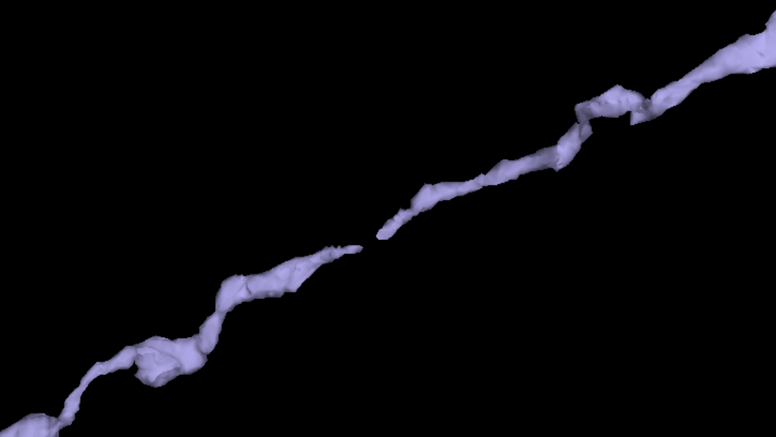
Fig. 51 Example of a continuous neuron whose mesh has a gap.#
Many meshes are not actually fully continuous due to small gaps in the segmentation. However, information collected during proofreading allows one to partially repair these gaps by adding in links where the segmentation was merged across a small gap. If you are just visualizing a mesh, these gaps are not a problem, but if you want to do analysis on the mesh, you will want to heal these gaps. Conveniently, there’s a function to do this:
mesh.add_link_edges(
    seg_id=root_id, # This needs to be the same as the root id used to download the mesh
    client=client.chunkedgraph,
)
Properties#
Meshes have a large number of properties, many of which come from being based on the Trimesh library’s mesh format, and others being specific to MeshParty.
Several of the most important properties are:
mesh.vertices: AnN x 3list of vertices and their 3d location in nanometers, whereNis the number of vertices.mesh.faces: AnP x 3list of integers, with each row specifying a triangle of connected vertex indices.mesh.edges: AnM x 2list of integers, with each row specifying a pair of connected vertex indices based off of faces.mesh.edges: AnM x 2list of integers, with each row specifying a pair of connected vertex indices based off of faces.mesh.link_edges: AnM_l x 2list of integers, with each row specifying a pair of “link edges” that were used to heal gaps based on proofreading edits.mesh.graph_edges: An(M+M_l) x 2list of integers, with each row specifying a pair of graph edges, which is the collection of bothmesh.edgesandmesh.link_edges.mesh.csgraph: A Scipy Compressed Sparse Graph representation of the mesh as anNxNgraph of vertices connected to one another using graph edges and with edge weights being the distance between vertices. This is particularly useful for computing shortest paths between vertices.mesh.nxgraph: a networkx graph object
Important
EM meshes are not generally “watertight”, a property that would enable a number of properties to be computed natively by Trimesh. Because of this, Trimesh-computed properties relating to solid forms or volumes like mesh.volume or mesh.center_mass do not have sensible values and other approaches should be taken. Unfortunately, because of the Trimesh implementation of these properties it is up to the user to be aware of this issue.
Visualization#
There are a variety of tools for visualizing meshes in python. MeshParty interfaces with VTK, a powerful but complex data visualization library that does not always work well in python. The basic pattern for MeshParty’s VTK integration is to create one or more “actors” from the data, and then pass those to a renderer that can be displayed in an interactive approach. The following code snippet shows how to visualize a mesh using this approach.
mesh_actor = trimesh_vtk.mesh_actor(
  mesh,
  color=(1,0,0),
  opacity=0.5,
)
trimesh_vtk.render_actors([mesh_actor])
Note that by default, neurons will appear upside down because the coordinate system of the dataset has the y-axis value increasing along the “downward” pia to white matter axis. More documentation on the MeshParty VTK visualization can be found here.
Other tools worth exploring are PyVista, Polyscope, Vedo, MeshLab, and if you have some existing experience, Blender (see Blender integration by our friends behind Navis, a fly-focused framework analyzing connectomics data).
Masking#
One of the most common operations on meshes is to mask them to a particular region of interest.
This can be done by “masking” the mesh with a boolean array of length N where N is the number of vertices in the mesh, with True where the vertex should be kept and False where it should be omitted.
There are several convenience functions to generate common masks in the Mesh Filters module.
In the following example, we will first mask out all vertices that aren’t part of the largest connected component of the mesh (i.e. get rid of floating vertices that might arise due to internal surfaces) and then mask out all vertices that are more than 20,000 nm away from the soma center.
from meshparty import mesh_filters

root_id =864691135492614239
root_point = client.materialize.tables.nucleus_detection_v0(pt_root_id=root_id).query()['pt_position'].values[0] * [4,4,40]  # Convert the nucleus location from voxels to nanometers via the data resolution.

mesh = mm.mesh(seg_id=root_id)
# Heal gaps in the mesh
mesh.add_link_edges(
    seg_id=root_id,
    client=client.chunkedgraph,
)

# Generate and use the largest component mask
comp_mask = mesh_filters.filter_largest_component(mesh)
mask_filt = mesh.apply_mask(comp_mask)

soma_mask = mesh_filters.filter_spatial_distance_from_points(
    mask_filt,
    root_point,
    20_000, # Note that this is in nanometers
)
mesh_soma = mesh.apply_mask(soma_mask)
This resulting mesh is just a small cutout around the soma.
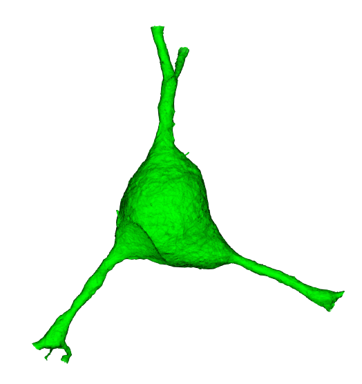
Fig. 52 Soma cutout from a full-neuron mesh.#
Working with Meshwork Files#
Loading a meshwork file imports the level 2 graph (the “mesh”), the skeleton, and a collection of associated annotations.
from meshparty import meshwork
nrn = meshwork.load_meshwork(mesh_filename)
The main three properties of the meshwork object are:
nrn.mesh : The l2graph representation of the reconstruction.
nrn.skeleton : The skeleton representation of the reconstruction.
nrn.anno : A table of annotation dataframes and associated metadata that links them to specific vertices in the mesh and skeleton.
Meshwork nrn.mesh vs nrn.skeleton#
Skeletons are “tree-like”, where every vertex (except the root vertex) has a single parent that is closer to the root than it, and any number of child vertices. Because of this, for a skeleton there are well-defined directions “away from root” and “towards root” and few types of vertices have special names:
Branch point: vertices with two or more children, where a neuronal process splits.
End point: vertices with no children, where a neuronal process ends.
Root point: The one vertex with no parent node. By convention, we typically set the root vertex at the cell body, so these are equivalent to “away from soma” and “towards soma”.
Segment: A collection of vertices along an unbranched region, between one branch point and the next end point or branch point downstream.
Visit the EM Skeletons page see more about skeletons, how to generate them, and how to work with them.
Meshes are arbitrary collections of vertices and edges, but do not have a notion of “parent” or “child” “branch point” or “end point”. Here, this means the “mesh” used here includes a vertex for every level 2 chunk, even where it is thick like at a cell body or very thick dendrite. However, by default this means that there is not always a well-defined notion of parent or child nodes, or towards or away from root.
In contrast “Meshes” (really, graphs of connected vertices) do not have a unique “inward” and “outward” direction. For the sake of rapid skeletonization, the “meshes” we use here are really the graph of level 2 vertices as described above. These aren’t a mesh in the visualization sense of the section on downloading Meshes, but have the same data representation.
To handle this, the meshwork object associates each mesh vertices with a single nearby skeleton vertex, and each skeleton vertex is associated with one or more mesh vertices. By representing data this way, annotations like synapses can be directly associated with a mesh vertex (because synapses can be anywhere on the object) and then mapped to the skeleton in order to enjoy the topological benefits of the skeleton representation.
# By the definition of skeleton vs mesh, we would expect that mesh contains more vertices than the skeleton.
# We can see this by looking at the size of the skeleton vertex location array vs the size of the mesh vertex location array.

print('Skeleton vertices array length:', len(nrn.skeleton.vertices))
print('Mesh vertices array length:', len(nrn.mesh.vertices))
#Let us try to visualize the skeleton:
# Visualize the whole skeleton

# here's a simple way to plot vertices of the skeleton
import matplotlib.pyplot as plt
from mpl_toolkits import mplot3d
%matplotlib notebook

fig = plt.figure(figsize=(6, 6))
ax = plt.axes(projection='3d')
ax.scatter3D(nrn.skeleton.vertices[:,0], nrn.skeleton.vertices[:,1], nrn.skeleton.vertices[:,2], s=1)
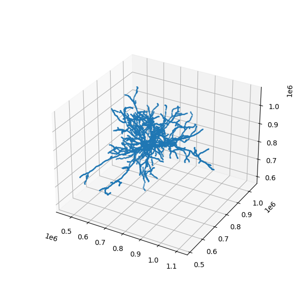
Fig. 53 Scatterplot of skeleton vertices as a point cloud.#