
Skeletons#
Important
Before using any programmatic access to the data, you first need to set up your CAVEclient token.
Often in working with neurons, you want to measure things along a linear dimension of a neuron. Length of axon, for example. Or number of branches. However, the EM segmentation is a complex 3d shape that makes this non-trivial.
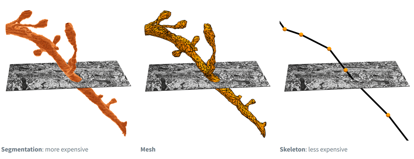
Fig. 47 Electron microscopy data can be represented and rendered in multiple formats, at different levels of abstraction from the original imagery#
There are methods for reducing the shape of a segmented neuron down to a linear tree-like structure usually referred to as a skeleton. We have precalculated skeletons for a large number of cells in the MICrONS dataset, including the proofread cells with the most complete axons.
There are several formats of EM skeleton that you may encounter in this workshop and tutorial material. See the subsections below for more about them. As a summary:
swc skeleton : files end in .swc
meshwork skeleton : objects saved in h5 file format
precomputed skeleton : a binary file for each skeleton, within a directory with metadata ‘info’ files on how to render them
All of these formats are composed of a set of vertices and edges which form the graph of the neuron’s branching structure. As well as information about the compartment type of the vertex, indicating if it is axon, dendrite, soma etc. And the radius of the branch, measured as half the cable thickness in micrometers.
However, the different formats may have different metadata attached to each vertex. Meshwork skeleton objects may include annotations about the input and output synapses, and provide functions to operate on the graph of the skeleton. Precomputed format may include arbitrary vertex properties that summarize connectivity information (for EM neurons) and CCF brain area (for exaSPIM neurons; see the section on Single Cell Morphology for more)
Note
Any format of skeleton can be converted into a Meshwork skeleton object to make use of the graph functions.
Dataset specificity#
The examples below are written with the MICrONS dataset. To access the V1DD dataset change the datastack from minnie65_public to v1dd_public
What is a Precomputed skeleton?#
These skeletons are stored in the cloud as a bytes-IO object, which can be viewed in Neuroglancer, or downloaded with CAVEclient.skeleton module. These precomputed skeletons also contain annotations on the skeletons that have the synapses, which skeleton nodes are axon and which are dendrite, and which are likely the apical dendrite of excitatory neurons.
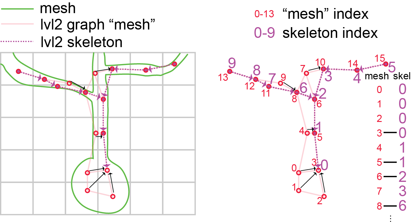
Fig. 48 Cartoon illustration of “level 2” graph and skeletons.#
The precomputed format is flexible and scalable, applies for EM data and light microscopy data, and can be rendered in Neuroglancer.
For more on how skeletons are generated from the mesh objects see the section below, and for additional tools for generating, cacheing, and downloading meshes, see the Skeleton Service documentation
CAVEclient to download skeletons#
Retrieve a skeleton using get_skeleton(). The available output_formats (described below) are:
dictcontaining vertices, edges, radius, compartment, and various metadata (default if unspecified)swca Pandas Dataframe in the SWC format, with ordered vertices, edges, compartment labels, and radius.
Note: if the skeleton doesn’t exist in the server cache, it may take 20-60 seconds to generate the skeleton before it is returned. This function will block during that time. Any subsequent retrieval of the same skeleton should go very quickly however.
from caveclient import CAVEclient
import numpy as np
import pandas as pd

client = CAVEclient("minnie65_public")

# Example: pyramidal cell in v1507
example_cell_id = 864691135572530981
# Download as 'SWC' fromat

sk_df = client.skeleton.get_skeleton(example_cell_id, output_format='swc')

sk_df.head()
| id | type | x | y | z | radius | parent | |
|---|---|---|---|---|---|---|---|
| 0 | 0 | 1 | 1365.120 | 763.456 | 812.60 | 3.643 | -1 |
| 1 | 1 | 3 | 1368.200 | 755.760 | 811.24 | 0.300 | 0 |
| 2 | 2 | 3 | 1368.200 | 758.552 | 811.68 | 1.915 | 1 |
| 3 | 3 | 3 | 1368.200 | 758.560 | 812.12 | 1.915 | 2 |
| 4 | 4 | 3 | 1368.192 | 758.560 | 812.44 | 2.815 | 3 |
Skeletons are “tree-like”, where every vertex (except the root vertex) has a single parent that is closer to the root than it, and any number of child vertices. Because of this, for a skeleton there are well-defined directions “away from root” and “towards root” and few types of vertices have special names:
You can see these vertices and edges represented in the alternative dict skeleton output.
sk_dict = client.skeleton.get_skeleton(example_cell_id, output_format='dict')

sk_dict.keys()
dict_keys(['meta', 'edges', 'mesh_to_skel_map', 'root', 'vertices', 'compartment', 'radius', 'lvl2_ids'])
Alternately, you can query a set of root_ids, for example all of the proofread cells in the dataset, and bulk download the skeletons
prf_root_ids = client.materialize.tables.proofreading_status_and_strategy(
    status_axon='t').query()['pt_root_id']
prf_root_ids.head(3)
0    864691136195824204
1    864691135701896315
2    864691135136188185
Name: pt_root_id, dtype: int64
convert dictionary to meshwork skeleton#
We use the python package Meshparty to convert between mesh representations of neurons, and skeleton representations.
Skeletons are “tree-like”, where every vertex (except the root vertex) has a single parent that is closer to the root than it, and any number of child vertices. Because of this, for a skeleton there are well-defined directions “away from root” and “towards root” and few types of vertices have special names:
Converting the pregenerated skeleton sk_dict to a meshwork object sk converts the skeleton to a graph object, for convenient representation and analysis.
from meshparty.skeleton import Skeleton

sk = Skeleton.from_dict(sk_dict)
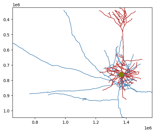
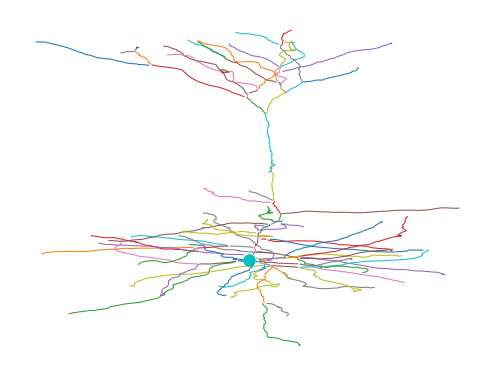
Plot with skeleton_plot#
Our convenience package skeleton_plot renders the skeleton in aligned, 2D views.
pip install skeleton_plot
Our convenience package skeleton_plot renders the skeleton in aligned, 2D views, with the compartments labeled in different colors. Here, dendrite is red, axon is blue, and soma (the root of the connected graph) is olive
from skeleton_plot.plot_tools import plot_skel

plot_skel(sk=sk,
          invert_y=True,
          pull_compartment_colors=True,
          plot_soma=True,
         )
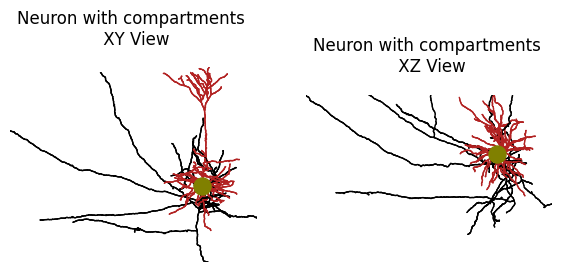
Skeleton plot is is wrapped around matplotlib, and can be treated as any other subplot. There are arguments to adjust the compartment colors and 2D projection direction.
import matplotlib.pyplot as plt
%matplotlib inline

f, ax = plt.subplots(1,2, figsize=(7, 10))

# Coronal view
plot_skel(
    sk,
    title="Neuron with compartments \n XY View",
    line_width=1,
    plot_soma=True,
    soma_size = 150,
    invert_y=True,
    pull_compartment_colors=True,
    x="x",
    y="y",
    skel_color_map = { 1: "olive", 2: "black", 3: "firebrick",4: "salmon", },
    ax=ax[0],
)

# top down view
plot_skel(
    sk,
    title="Neuron with compartments \n XZ View",
    line_width=1,
    plot_soma=True,
    soma_size = 150,
    invert_y=True,
    pull_compartment_colors=True,
    x="x",
    y="z",
    skel_color_map = { 1: "olive", 2: "black", 3: "firebrick",4: "salmon", },
    ax=ax[1],
)

for aa in ax:
    aa.spines['right'].set_visible(False)
    aa.spines['left'].set_visible(False)
    aa.spines['top'].set_visible(False)
    aa.spines['bottom'].set_visible(False)
    aa.axis('off')
Working with Meshwork Objects#
Skeletons are “tree-like”, where every vertex (except the root vertex) has a single parent that is closer to the root than it, and any number of child vertices. Because of this, for a skeleton there are well-defined directions “away from root” and “towards root” and few types of vertices have special names:
Branch point: vertices with two or more children, where a neuronal process splits.
End point: vertices with no children, where a neuronal process ends.
Root point: The one vertex with no parent node. By convention, we typically set the root vertex at the cell body, so these are equivalent to “away from soma” and “towards soma”.
Segment: A collection of vertices along an unbranched region, between one branch point and the next end point or branch point downstream.
Skeleton Properties and Methods#
To plot this skeleton in a more sophisticated way, you have to start thinking of it as a graph, and the meshwork object has a bunch of tools and properties to help you utilize the skeleton graph.
Let’s list some of the most useful ones below You access each of these with nrn.skeleton.* Use the ? to read more details about each one
Properties
branch_points: a list of skeleton vertices which are branchesroot: the skeleton vertex which is the somadistance_to_root: an array the length of vertices which tells you how far away from the root each vertex isroot_position: the position of the root node in nanometersend_points: the tips of the neuroncover_paths: a list of arrays containing vertex indices that describe individual paths that in total cover the neuron without repeating a vertex. Each path starts at an end point and continues toward root, stopping once it gets to a vertex already listed in a previously defined path. Paths are ordered to start with the end points farthest from root first. Each skeleton vertex appears in exactly one cover path.csgraph: a scipy.sparse.csr.csr_matrix containing a graph representation of the skeleton. Useful to do more advanced graph operations and algorithms. https://docs.scipy.org/doc/scipy/reference/sparse.csgraph.htmlkdtree: a scipy.spatial.ckdtree.cKDTree containing the vertices of skeleton as a kdtree. Useful for quickly finding points that are nearby. https://docs.scipy.org/doc/scipy/reference/generated/scipy.spatial.cKDTree.html
Methods
path_length(paths=None): the path length of the whole neuron if no arguments, or pass a list of paths to get the path length of that. A path is just a list of vertices which are connected by edges.path_to_root(vertex_index): returns the path to the root from the passed vertexpath_between(source_index, target_index): the shortest path between the source vertex index and the target vertex indexchild_nodes(vertex_indices): a list of arrays listing the children of the vertex indices passed inparent_nodes(vertex_indices): an array listing the parent of the vertex indices passed in
Vertices and Neighborhoods#
# Vertices
print(f"There are {len(sk.vertices)} vertices in this neuron", "\n")

# Branch points
print("Branch points are at the following vertices: \n",sk.branch_points, "\n")

# End points
print("End points are at the following vertices: \n",sk.end_points, "\n")

# Root - the point associated with the root node, which is the soma
print("Root is vertex: ", sk.root.item(), "\n")

# Select downstream nodes from one branch point
downstream_nodes = sk.downstream_nodes(sk.branch_points[3])
print("Nodes downstream of selected brach are: \n", downstream_nodes, "\n")
There are 7445 vertices in this neuron

Branch points are at the following vertices:
 [ 253  987 1483 1701 1762 1933 2323 2567 2616 2634 2636 2845 2921 3090
 3252 3280 3381 3413 3446 3603 3625 3630 3631 3683 3711 3783 3821 3848
 3871 3894 3930 3932 3962 4020 4023 4054 4116 4122 4125 4127 4130 4187
 4225 4230 4233 4245 4250 4255 4413 4434 4455 4473 4479 4482 4523 4536
 4629 4762 4800 4830 4831 4832 4933 4934 4963 5060 5077 5104 5118 5123
 5128 5132 5145 5151 5194 5277 5341 5357 5359 5627 5686 5692 5693 5743
 5767 6182 6273 6294 6570 6607 7371 7444]

End points are at the following vertices:
 [   0   98  260  268  464  924 1265 1282 1364 1391 1415 1442 1448 1497
 1568 1622 1659 1728 1744 1758 1825 2043 2054 2102 2273 2357 2384 2407
 2533 2534 2565 2617 2665 2703 2756 2768 2823 2850 3062 3102 3175 3275
 3344 3379 3534 3550 3562 3762 3846 3906 3928 4192 4362 4370 4374 4606
 4658 4783 4851 5004 5278 5313 5396 5398 5454 5478 5481 5721 5801 5825
 6330 6335 6413 6461 6725 6776 6829 6836 6890 6945 7041 7098 7109 7137
 7167 7169 7234 7263 7265 7272 7282 7321 7340 7360 7366 7376 7388 7438]

Root is vertex:  7444

Nodes downstream of selected brach are:
 [ 464  468  473  474  475  476  481  482  483  489  490  495  496  502
  503  509  513  514  518  519  520  521  525  526  527  528  529  530
  535  536  542  543  547  548  552  553  559  563  564  565  569  570
  571  572  573  578  579  580  581  586  587  588  589  590  594  595
  596  597  598  599  600  605  606  607  613  614  615  616  620  621
  622  623  624  625  630  631  632  633  634  635  636  637  638  639
  640  641  648  649  650  654  655  656  657  658  659  660  661  662
  663  664  665  670  671  672  673  674  675  676  682  683  688  689
  690  694  700  701  705  706  711  715  716  717  723  724  729  730
  731  732  737  738  739  740  745  746  747  748  753  754  758  759
  765  766  771  772  777  778  782  783  788  789  794  795  799  800
  804  809  810  815  819  820  821  827  828  829  830  831  836  837
  838  839  840  841  846  847  853  854  855  859  860  861  862  867
  868  873  874  875  876  877  881  882  883  884  885  886  890  891
  896  897  902  903  904  911  912  925  926  934  935  936  944  945
  946  947  952  953  954  955  956  957  964  965  966  975  976  990
  991  992 1003 1004 1011 1012 1013 1021 1031 1032 1037 1038 1046 1047
 1051 1056 1057 1062 1063 1068 1069 1076 1077 1078 1079 1083 1084 1091
 1092 1096 1097 1102 1103 1107 1108 1109 1113 1118 1119 1120 1126 1130
 1131 1135 1136 1142 1143 1147 1148 1149 1153 1154 1158 1165 1166 1170
 1171 1176 1180 1181 1186 1190 1191 1192 1196 1197 1202 1203 1204 1205
 1210 1211 1212 1217 1218 1219 1223 1228 1229 1234 1235 1239 1240 1241
 1242 1246 1250 1251 1255 1256 1260 1266 1267 1268 1274 1275 1281 1288
 1299 1307 1308 1316 1323 1325 1334 1342 1343 1351 1352 1360 1371 1372
 1382 1383 1393 1394 1395 1405 1406 1419 1420 1421 1432 1447 1448 1449
 1450 1464 1465 1466 1467 1468 1483 1500 1515 1516 1536 1537 1555 1572
 1573 1595 1596 1616 1639 1640 1672 1673 1696 1697 1698 1699 1700 1701
 1722 1723 1725 1751 1784 1826 1857 1858 1885 1886 1917 1944 1945 1968
 1969 1970 1971 1972 1973 1977 1995 1996 1997 1998 1999 2000 2001 2002
 2005 2007 2024 2026 2030 2032 2033 2035 2037 2065 2066 2067 2068 2072
 2073 2074 2075 2076 2112 2113 2114 2119 2150 2152 2153 2154 2156 2189
 2191 2192 2193 2194 2225 2226 2227 2228 2229 2231 2232 2233 2235 2267
 2268 2269 2270 2305 2306 2307 2308 2309 2310 2311 2351 2352 2393 2394
 2395 2451 2452 2453 2454 2455 2456 2457 2500 2501 2502 2503 2544 2545
 2546 2547 2548 2549 2550 2551 2552 2553 2554 2555 2605 2606 2607 2608
 2609 2610 2611 2612 2613 2614 2615 2616 2617 2618 2665 2667 2669 2670
 2672 2674 2676 2678 2679 2680 2681 2682 2684 2686 2688 2689 2690 2691
 2692 2693 2694 2696 2697 2698 2699 2701]
Paths and Segments#
# Segments - path of nodes between two vertices i and j which are assumed to be a root, branch point, or endpoint.
print("The number of branch segments are: ",len(sk.segments), "\n")

# Path between - path_between() function finds the vertices on the path between two points on the skeleton graph.
nodes_between = sk.path_between(0,150)
print("Path between the given nodes: ", nodes_between, "\n")

# Path-length - path_length() function calculates the physical distance along the path for a neuron
full_pathlength = sk.path_length() / 1000 # Convert to microns
print("Path-length of the entire neuron: ", full_pathlength, ' um', "\n")

# Path-length for arbitrary segment
example_segment = 11
segment_pathlength = sk.path_length(sk.segments[example_segment]) / 1000 # Convert to microns
print("Path-length of one segment: ", segment_pathlength, ' um', "\n")
The number of branch segments are:  190

Path between the given nodes:  [  0   1   2   3   4   5   6   7   8   9  10  11  12  13  14  15  16  17
  18  19  20  21  22  23  24  25  26  27  29  28  30  31  32  33  34  35
  36  37  38  39  40  41  42  43  44  45  46  47  48  49  50  51  52  53
  54  55  56  57  58  59  60  61  62  63  64  65  66  67  68  69  70  71
  72  73  74  75  76  77  78  79  80  81  82  83  84  85  86  87  88  89
  90  91  92  93  94  95  96 100 101 103 106 108 109 112 115 117 118 120
 122 124 125 127 128 130 131 133 134 136 139 140 143 145 146 148 150]

Path-length of the entire neuron:  14846.251  um

Path-length of one segment:  408.098  um
Masking#
One of the most useful methods of the skeleton meshwork’s is the ability to mask or select only parts of the skeleton to work with at a time. The function apply_mask() acts on the meshwork skeleton, and will apply in place if apply_mask(in_place=True).
Warning: be aware when setting a mask in place–mask operations are additive. To reset the mask completely, use reset_mask(in_place=True).
# Let's select a set of nodes from example segment 11
example_segment = 11
selected_nodes = sk.segments[example_segment]
print("Path of the selected nodes is: \n", selected_nodes, "\n")

# reset to make sure you have the full skeleton
sk.reset_mask(in_place=True)

# Apply a mask to these nodes
sk_masked = sk.apply_mask(selected_nodes)

# Check that this masked skeleton matches the pathlength calculated above
print("Path-length of masked segment: ", sk_masked.path_length() / 1000, ' um')
Path of the selected nodes is:
 [1391 1403 1417 1430 1445 1444 1443 1462 1480 1496 1495 1511 1512 1532
 1531 1550 1567 1585 1607 1606 1627 1626 1658 1657 1688 1687 1713 1712
 1742 1774 1773 1813 1812 1842 1840 1872 1871 1903 1902 1934 1957 1956
 1986 2018 2058 2057 2105 2106 2148 2186 2187 2188 2230 2271 2312 2313
 2353 2396 2398 2459 2505 2506 2558 2560 2561 2623 2624 2625 2710 2711
 2712 2777 2778 2713 2714 2779 2781 2835 2837 2838 2909 2911 2976 3038
 3040 3121 3122 3208 3209 3211 3312 3314 3315 3316 3317 3416 3415 3418
 3517 3518 3598 3678 3761 3842 3844 3843 3925 3927 4016 4128 4129 4246
 4248 4354 4472 4469 4639 4641 4638 4817 4821 4820 4973 4974 5072 5168
 5268 5270 5365 5444 5528 5529 5604 5691 5690 5689 5776 5851 5918 5973
 6052 6119 6120 6193 6268 6270 6271 6329 6388 6390 6442 6445 6444 6446
 6498 6550 6551 6499 6501 6503 6553 6554 6597 6644 6645 6689 6743 6782
 6821 6822 6861 6892 6897 6936 6982 6983 6985 6938 6939 6899 6864 6865
 6826 6785 6786 6746 6747 6692 6649 6650 6604 6603 6558 6559 6510 6511
 6454 6396 6397 6398 6343 6285 6286 6212 6213 6140 6068 6069 5990 5991
 5935 5936 5874 5794 5796 5707 5626 5630 5629 5551 5552 5468 5390 5391
 5297 5298]

Path-length of masked segment:  408.098  um
Critically, apply_mask() allows us to mask a neuron according to its compartment label: axon, dendrite, soma, etc.
Compartment label conventions (from standardized swc files www.neuromorpho.org )
0 - undefined
1 - soma
2 - axon
3 - (basal) dendrite
4 - apical dendrite
5+ - custom
print("The unique compartment labels in this skeleton are:", np.unique(sk.vertex_properties['compartment']), "\n")

# Select the indices associated with the dendrites
dendrite_inds = (sk.vertex_properties['compartment']==3) | (sk.vertex_properties['compartment']==4)| (sk.vertex_properties['compartment']==1) #soma is included here to connect the dendrite graphs

# create new skeleton that masks (selects) only the axon
sk_dendrite = sk.apply_mask(dendrite_inds)
print("Dendrite pathlength of all branches is : ", sk_dendrite.path_length() / 1000, ' um', "\n")

# Select the indices associated with the axon, find length
axon_inds = sk.vertex_properties['compartment']==2
sk_axon = sk.apply_mask(axon_inds)
print("Axon pathlength is : ", sk_axon.path_length() / 1000, ' um', "\n")
The unique compartment labels in this skeleton are: [1 2 3]

Dendrite pathlength of all branches is :  7243.2455  um

Axon pathlength is :  7599.738  um
# Render all the segments in the dendrite graph

fig, ax = plt.subplots(figsize=(4,3), dpi=150)

for ss in range(len(sk_dendrite.segments)):
    seg = sk_dendrite.segments[ss]

    ax.plot(sk_dendrite.vertices[seg][:,0],
            sk_dendrite.vertices[seg][:,1], linewidth=0.5)

# add soma marker
ax.plot(sk.vertices[sk.root][0],
        sk.vertices[sk.root][1], 'oc', markersize=5)

ax.invert_yaxis()
ax.axis('off')
(1208623.6, 1519800.4, 958991.2, 291440.8)
How EM skeletons are generated#
Fig. 49 Cartoon illustration of “level 2” graph and skeletons.#
In order to understand how these skeletons have been made, you have to understand how large scale EM data is represented. Portions of 3d space are broken up into chunks, such as the grid in the image above. Neurons, such as the cartoon green cell above, span many chunks. Components of the segmentation that live within a single chunk are called level 2 ids, this is because in fact the chunks get iteratively combined into larger chunks, until the chunks span the whole volume. We call this the PyChunkedGraph or PCG, after the library which we use to store and interact with this representation. Level 0 is the voxels, level 1 refers to the grouping of voxels within the chunk (also known as supervoxels) and level 2 are the groups of supervoxels within a chunk. A segmentation result can be thought of as a graph at any of these levels, where the voxels, supervoxels, or level 2 ids that are part of the same object are connected. In the above diagram, the PCG level 2 graph is represented as the light red lines.
Such graphs are useful in that they track all the parts of the neuron that are connected to one another, but they aren’t skeletons, because the graph is not directed, and isn’t a simple branching structure.
In order to turn them into a skeleton we have to run an algorithm, that finds a tree like structure that covers the graph and gets close to every node. This is called the TEASAR algorithm and you can read more about how to skeletonize graphs in the MeshParty documentation.
The result of the algorithm, when applied to a level 2 graph, is a linear tree (like the dotted purple one shown above), where a subset of the level 2 chunks are vertices in that tree, but all the unused level 2 nodes “near” a vertex (red unfilled circles) on the graph are mapped to one of the skeleton vertices (black arrows). This means there are two sets of indices, mesh indices, and skeleton indices, which have a mapping between them (see diagram above).
The MeshParty library allows us to easily store these representations and helps us relate them to each other. A Meshwork object is a data structure that is designed to have three main components that are kept in sync with mesh and skeleton indices:
mesh: the graph of PCG level2 ID nodes that are skeletonized, stored as a standard meshparty mesh. Note that this is not the high resolution mesh that you see in neuroglancer. See EM Meshes for more
skeleton: a meshwork skeleton, derived from the simplification of the mesh
anno : is a class that holds dataframes and adds some extra info to keep track of indexing.