
Using Python to Access Neurodata Without Borders-type Files#
This tutorial will demonstrate the structure of the data file in a Neurodata Without Borders type (NWB) file and showcase how to access various parts of the data. We will use a specific example using an ecephys file, but the process is general.
We begin with package imports which we’ll need. hdmf_zarr handles the ZArray objects that appear in NWB files, while nwbwidgets will provide us with a useful tool down the line.
from hdmf_zarr import NWBZarrIO
from nwbwidgets import nwb2widget

%matplotlib inline
In order to do any analysis, of course, we’ll also need the usual libraries:
import numpy as np
import pandas as pd
import matplotlib.pyplot as plt
Accessing an NWB file#
To manipulate the data in the file, we will first need to find the file we’re interested in and then load it into Python. We assume here that we have already received the datafile somehow and we know what directory we’ve stored the file in, so we will simply path directly to the file (which is of file type .nwb.zarr).
mouse_id = '655565'

nwb_file = '/data/SWDB 2024 CTLUT data/ecephys_655565_2023-03-31_14-47-36_nwb/ecephys_655565_2023-03-31_14-47-36_experiment1_recording1.nwb.zarr'
So far, all we’ve done is find the path and store it as a string in Python. Now that we have the NWB file’s path, we still need to load it into Python, which we can do using NWBZarrIO.
with NWBZarrIO(nwb_file, "r") as io:
    nwbfile_read = io.read()
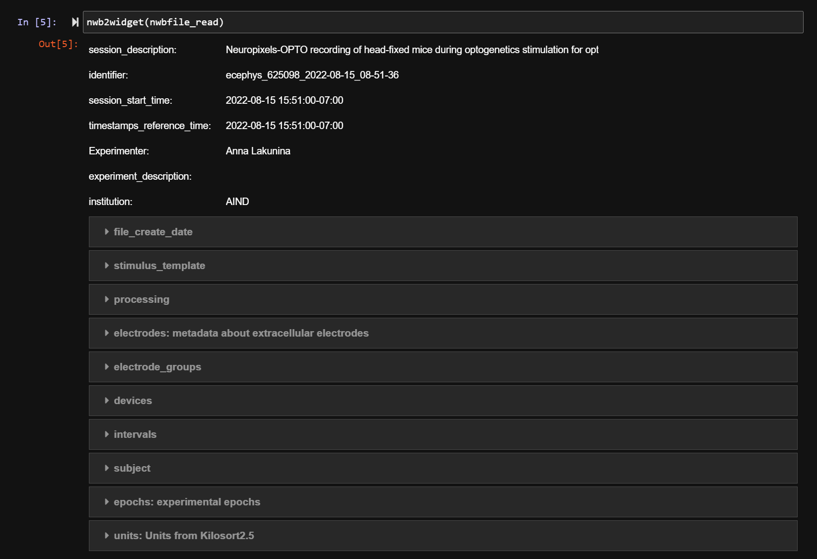
This stores all the information contained in the NWB file into a NWBFile object from the pynwb package, and now we’re ready to start working with the data. The first thing we might be interested in is just seeing the contents of the NWB file, which we can do by using the nwb2widget tool. Below, a screenshot of the output is included to show what information it contains:
nwb2widget(nwbfile_read);
The various types of data contained in the file when loaded into Python are simply attributes of the nwbfile_read object, which we access in the usual way nwbfile_read.*. Depending on the table of interest, they might be stored as different types of objects, however; for example, several are stored as objects specific to the pynwb package.
Now we will access the data directly.
print(nwbfile_read)
root pynwb.file.NWBFile at 0x140228460445120
Fields:
  devices: {
    ProbeA <class 'pynwb.device.Device'>,
    ProbeB <class 'pynwb.device.Device'>
  }
  electrode_groups: {
    ProbeA <class 'pynwb.ecephys.ElectrodeGroup'>,
    ProbeB <class 'pynwb.ecephys.ElectrodeGroup'>
  }
  electrodes: electrodes <class 'hdmf.common.table.DynamicTable'>
  epochs: epochs <class 'pynwb.epoch.TimeIntervals'>
  file_create_date: [datetime.datetime(2023, 5, 15, 21, 49, 33, 28522, tzinfo=tzutc())]
  identifier: ecephys_655565_2023-03-31_14-47-36
  intervals: {
    epochs <class 'pynwb.epoch.TimeIntervals'>,
    trials <class 'pynwb.epoch.TimeIntervals'>
  }
  processing: {
    behavior <class 'pynwb.base.ProcessingModule'>,
    ecephys <class 'pynwb.base.ProcessingModule'>
  }
  session_description: Neuropixels-OPTO recording of head-fixed mice during optogenetics stimulation for opto-tagging.
  session_start_time: 2023-03-31 14:47:36-07:00
  stimulus_template: {
    internal_blue-train-0.02mW <class 'pynwb.base.TimeSeries'>,
    internal_blue-train-0.04mW <class 'pynwb.base.TimeSeries'>,
    internal_blue-train-0.06mW <class 'pynwb.base.TimeSeries'>,
    internal_blue-train-0.08mW <class 'pynwb.base.TimeSeries'>,
    internal_blue-train-0.1mW <class 'pynwb.base.TimeSeries'>,
    internal_red-train-0.02mW <class 'pynwb.base.TimeSeries'>,
    internal_red-train-0.04mW <class 'pynwb.base.TimeSeries'>,
    internal_red-train-0.06mW <class 'pynwb.base.TimeSeries'>,
    internal_red-train-0.08mW <class 'pynwb.base.TimeSeries'>,
    internal_red-train-0.1mW <class 'pynwb.base.TimeSeries'>
  }
  subject: subject pynwb.file.Subject at 0x140228458827968
Fields:
  age: P158D
  age__reference: birth
  date_of_birth: 2022-10-24 00:00:00-07:00
  genotype: Chat-IRES-Cre-neo/Chat-IRES-Cre-neo
  sex: M
  species: Mus musculus
  subject_id: 655565

  timestamps_reference_time: 2023-03-31 14:47:36-07:00
  trials: trials <class 'pynwb.epoch.TimeIntervals'>
  units: units <class 'pynwb.misc.Units'>
Accessing Units Data#
Since this is an ecephys file, let’s first access the units. This is a DataFrame object that contains information about all of the sorted units in this experiment.
units = nwbfile_read.units[:]
print(type(units))
<class 'pandas.core.frame.DataFrame'>
Let’s examine what information is stored in the DataFrame:
print(units.columns.values)
['spike_times' 'electrodes' 'waveform_mean' 'waveform_sd' 'unit_name'
 'drift_ptp' 'snr' 'isi_violations_ratio' 'default_qc' 'ks_unit_id'
 'l_ratio' 'half_width' 'repolarization_slope' 'sliding_rp_violation'
 'drift_mad' 'peak_trough_ratio' 'presence_ratio' 'rp_contamination'
 'recovery_slope' 'num_spikes' 'isolation_distance' 'device_name'
 'rp_violations' 'amplitude' 'amplitude_cutoff' 'peak_to_valley'
 'firing_rate' 'drift_std' 'd_prime' 'noise_label' 'peak_channel'
 'internal_blue_train_best_site' 'internal_blue_train_mean_latency'
 'internal_blue_train_mean_jitter' 'internal_blue_train_mean_reliability'
 'internal_blue_train_num_sig_pulses_paired'
 'internal_blue_train_channel_diff' 'internal_red_train_best_site'
 'internal_red_train_mean_latency' 'internal_red_train_mean_jitter'
 'internal_red_train_mean_reliability'
 'internal_red_train_num_sig_pulses_paired'
 'internal_red_train_channel_diff' 'predicted_cell_type']
Here, we can see the full list of columns stored in our DataFrame:
spike_times- spike times (in seconds) for the entire sessionelectrodes- electrode indices used for mean waveformwaveform_mean- mean spike waveform across all electrodeswaveform_sd- standard deviation of the spike waveform across all electrodesunit_name- universally unique identifier for this unitdefault_qc-Trueif this unit passes default quality control criteria,Falseotherwisepresence_ratio- fraction of the session for which this unit was present (default threshold = 0.8)num_spikes- total number of spikes detectedsnr- signal-to-noise ratio of this unit’s waveform (relative to the peak channel)isi_violations_ratio- metric that quantifies spike contamination (default threshold = 0.5)firing_rate- average firing rate of the unit throughout the sessionisolation_distance- distance to nearest cluster in Mahalanobis space (higher is better)l_ratio- related to isolation distance; quantifies the probability of cluster membership for each spikedevice_name- name of the probe that detected this unitamplitude_cutoff- estimated fraction of missed spikes (default threshold = 0.1)peak_trough_ratio- ratio of the max (peak) to the min (trough) amplitudes (based on 1D waveform)repolarization_slope- slope of return to baseline after trough (based on 1D waveform)amplitude- peak-to-trough distance (based on 1D waveform)d_prime- classification accuracy based on LDA (higher is better)recovery_slope- slope of return to baseline after peak (based on 1D waveform)half_width- width of the waveform at half the trough amplitude (based on 1D waveform)ks_unit_id- unit ID assigned by Kilosort
Note that the columns may vary from experiment to experiment, so it’s a good idea to check what columns are stored in any NWB file that you open. For instance, this file contains the above standard columns that appear in most NWB files from the Allen Institute, but also many more columns detailing the unit’s response to laser stimulation. These columns are further explained in the cell type lookup table tutorials.
To access data from a specific unit, we look at the row corresponding to that unit:
print(units.loc[418])
spike_times                                  [810.0001255327663, 869.9232313798699, 915.734...
electrodes                                   [768, 769, 770, 771, 772, 773, 774, 775, 776, ...
waveform_mean                                [[0.0, 0.0, 0.0, 0.0, 0.0, 0.0, 0.0, 0.0, 0.0,...
waveform_sd                                  [[0.0, 0.0, 0.0, 0.0, 0.0, 0.0, 0.0, 0.0, 0.0,...
unit_name                                                 f6e38bca-33ba-48cc-af02-75a27f42b7ed
drift_ptp                                                                                  NaN
snr                                                                                   6.655138
isi_violations_ratio                                                                       0.0
default_qc                                                                               False
ks_unit_id                                                                                31.0
l_ratio                                                                               0.149023
half_width                                                                            0.000243
repolarization_slope                                                             313290.923614
sliding_rp_violation                                                                       NaN
drift_mad                                                                                  NaN
peak_trough_ratio                                                                    -0.330413
presence_ratio                                                                        0.644231
rp_contamination                                                                           0.0
recovery_slope                                                                   -38637.486587
num_spikes                                                                               258.0
isolation_distance                                                                  141.030751
device_name                                                                             ProbeB
rp_violations                                                                              0.0
amplitude                                                                            69.265793
amplitude_cutoff                                                                           NaN
peak_to_valley                                                                        0.000607
firing_rate                                                                           0.041214
drift_std                                                                                  NaN
d_prime                                                                               4.067442
noise_label                                                                               good
peak_channel                                                                              38.0
internal_blue_train_best_site                                                              1.0
internal_blue_train_mean_latency                                                           NaN
internal_blue_train_mean_jitter                                                            NaN
internal_blue_train_mean_reliability                                                       0.0
internal_blue_train_num_sig_pulses_paired                                                  0.0
internal_blue_train_channel_diff                                                          28.0
internal_red_train_best_site                                                               1.0
internal_red_train_mean_latency                                                            NaN
internal_red_train_mean_jitter                                                             NaN
internal_red_train_mean_reliability                                                        0.0
internal_red_train_num_sig_pulses_paired                                                   0.0
internal_red_train_channel_diff                                                           28.0
predicted_cell_type                                                                   untagged
Name: 418, dtype: object
To look at the spike times for a specific unit, we look at the corresponding attribute of that unit.
print(units.loc[418]['spike_times'])
[ 810.00012553  869.92323138  915.73428283  993.46186793 1083.97800103
 1084.37176786 1089.61893294 1092.82656648 1096.59626237 1104.08294017
 1122.70730282 1125.34041942 1126.51636438 1129.27679993 1149.56591895
 1154.20855116 1166.86327015 1173.91335363 1176.37448709 1180.12824315
 1204.58823002 1218.85226241 1235.82063975 1235.83637457 1236.31450614
 1242.08294837 1244.65159236 1249.26466788 1249.44521834 1250.3503856
 1258.15654467 1258.88936281 1260.35690467 1260.36043833 1260.48044971
 1261.91264978 1261.91925041 1261.97372225 1262.13907127 1262.75761444
 1263.24219374 1263.75474236 1277.79954127 1282.3000847  1285.1322865
 1285.13595351 1292.74120776 1293.51769891 1297.33662557 1297.97231912
 1298.25296356 1298.98861539 1300.32024153 1301.9289663  1302.22299133
 1302.30006531 1307.71993123 1309.20901687 1309.72016916 1313.03775052
 1313.70558054 1320.65798737 1320.83285661 1324.20961025 1327.55279404
 1328.05610845 1342.03298021 1359.71812328 1364.14748767 1364.89158035
 1365.69926807 1366.36942043 1371.50374046 1375.13657435 1376.17882736
 1383.53526109 1389.51088072 1392.3238807  1394.06714595 1398.07691706
 1403.59520718 1405.08142334 1423.03552524 1423.7037959  1429.79206571
 1430.82366349 1431.01634842 1432.52099105 1433.25349382 1439.23120009
 1450.29651494 1451.11632593 1452.02093948 1455.97412463 1458.76341698
 1459.3572349  1461.10636737 1461.22491681 1461.800438   1467.17078004
 1468.11733638 1475.5309053  1477.01933862 1483.13582225 1484.99670197
 1488.51950543 1495.57367055 1505.52824486 1512.58018    1513.52840468
 1526.67538277 1527.18216414 1536.1034098  1544.84723864 1546.43738802
 1547.5140566  1551.91157495 1570.22131056 1570.83133279 1572.09928858
 1574.95555679 1579.42628029 1598.73067968 1600.77873627 1601.49757529
 1608.83166576 1612.36129514 1613.34382651 1613.56541417 1618.98289402
 1619.33949446 1627.02318305 1627.26987307 1629.81415336 1629.81755368
 1632.21151379 1637.66412367 1639.55353586 1650.90761066 1651.40935815
 1652.60833832 1654.73333947 1663.87067942 1686.98349232 1687.56674753
 1706.13920563 1712.22841537 1712.59144974 1721.0698736  1729.05084114
 1746.64462621 1748.49174811 1770.8974024  1776.49069853 1780.78503838
 1791.22689348 1794.01994108 1807.25139273 1824.05411554 1860.79957934
 1864.15286343 1865.37295748 1870.81732763 1871.24219086 1874.10090512
 1877.87989618 1890.09756301 1893.42628795 1937.31827045 1940.88666747
 1958.08006057 1966.77187749 1984.55029789 1989.71185282 1994.12430356
 2035.57325862 2079.8236104  2152.69883064 2166.64304108 2176.93501333
 2179.53132526 2204.94333605 2216.45245735 2246.74960844 2312.93004417
 2323.66347676 2332.03116466 2333.87475743 2342.75704456 2469.84298321
 2496.84616332 2573.61715125 2575.35928427 2582.88982898 2597.59004854
 2627.90130553 2629.5536326  2681.47160829 2690.96032946 2728.1732424
 2774.93925716 2800.31415257 2897.06914162 2905.85971618 2993.41622006
 3047.91182762 3138.28118603 3245.08149447 3250.41785293 3363.26069072
 3387.77985606 3405.24801557 3407.52443017 3441.21304865 3512.37734341
 3545.65351588 3602.1433092  3617.53372792 3703.08445952 3760.20331083
 3762.32128877 3813.95522977 3894.53797467 3958.05176217 4154.07333751
 4173.0556874  4180.58816869 4554.33138094 4572.91709499 4593.90613711
 4611.37661788 4681.01370214 4712.23169268 4847.82922662 4864.65831202
 5136.32570464 5374.39409871 5411.34026029 5411.58945041 5507.19160087
 5637.8718524  5649.97855918 5691.0316201  5722.23669494 5833.59971206
 6002.35099841 6015.55426634 6027.48486453 6059.7740764  6132.44734576
 6150.05200268 6233.31800264 6237.41204837 6319.09460545 6400.86718164
 6529.5848741  6636.06779153 6678.74083936]
We can also see how many spike times there are for a specific unit, which will tell us the number of spikes and allow us to access the time of a specific spike (in this case, accessing the time of the 189th spike):
print(len(units.loc[418]['spike_times']))
print(units.loc[418]['spike_times'][188])
258
2342.7570445621095
A useful sanity check here might also to be to ensure that the number of spike times matches the actual number of spikes recorded in the units table:
print(units.loc[418]['num_spikes'])
print(units.loc[418]['num_spikes'] == len(units.loc[418]['spike_times']))
258.0
True
So we can see that every recorded spike also has its time recorded, as we would expect. As another example, it is also possible to access and plot the waveform for a specific unit. Accessing the waveform is done in the same manner as accessing the spike times; in this case, we are interested in looking at ‘waveform_mean’ (note that here, we access it in two different ways: as an attribute of the units table, and as an element of the DataFrame). This is stored as a basic Python array. We can take a look at its dimensions to make sense of what data is stored here:
print(np.array(units.loc[418]['waveform_mean']).shape)
(210, 384)
Equipped with our knowledge of Neuropixels, we can see then that the dimensions are (time, channel). We can plot this to visualize each channel’s recordings over time. Note that due to the way that plt.imshow functions, we will need to take the transpose of the array to plot time on the x-axis. Also note that waveform_mean centers the times around the time of the spike.
plt.imshow(units.loc[418]['waveform_mean'].T, origin='lower')
plt.ylabel("Electrode")
plt.xlabel("Time (us)")
plt.show()
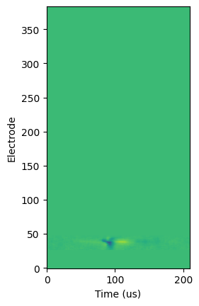
From above, we can see that most of the channels recorded the same values over time; the channel’s recording at any given time is indicated by the color of the plot at that time. Since most horizontal lines we can draw on this plot are monochromatic, we can conclude that the channel in question did not record any interesting variation in electric potential.
However, there is something interesting happening on channels 20 to 50!
We can plot the shape of the potential over time on those channels. Now, instead of a three-dimensional plot, we will have a two-dimensional plot of voltage over time, with each distinct line representing a different channel:
plt.plot(units.waveform_mean.loc[418][:,20:50])
plt.ylabel("uV")
plt.xlabel("Time (us)")
plt.show()
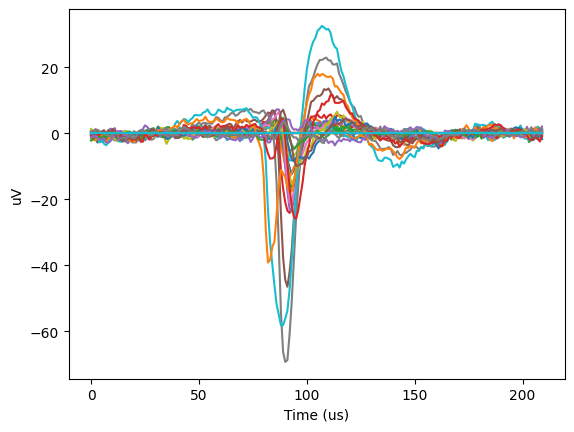
This has somthing interesting going on; we can clearly see the classic shape of an action potential, but it appears to be overlaid on some baseline sinusoidal oscillation in the voltage.
Moving on from the units table, let’s examine more of the data contained in the NWB file.
Accessing Trials Data#
The trials table includes information on the timing and experimental parameters for each trial conducted in the experiment. It can be accessed in the same way as the units table; again, this is a DataFrame object.
trials = nwbfile_read.trials[:]
print(trials.columns.values)
['start_time' 'stop_time' 'site' 'power' 'param_group' 'emission_location'
 'duration' 'rise_time' 'num_pulses' 'wavelength' 'type'
 'inter_pulse_interval' 'stimulus_template_name']
Notice that this is an example of an optotagging experiment from the Cell Type Look-Up Table (CTLUT) dataset, so the columns stored here are specific to that stimulus. Other NWB files for other experiments will have different column names pertaining to the stimulus or behavior used for that experiment. In this experiment, for example, we can see the length of the trials and the details on the lasers used as a stimulus.
Like with the units table, we can access a particular trial by asking for the row number (remember that these are indexed starting at 0):
print(trials.loc[1582])
start_time                             1696.596233
stop_time                              1696.646233
site                                            13
power                                          0.1
param_group                                  train
emission_location                           ProbeA
duration                                      0.01
rise_time                                    0.001
num_pulses                                       5
wavelength                                     638
type                                  internal_red
inter_pulse_interval                          0.04
stimulus_template_name    internal_red-train-0.1mW
Name: 1582, dtype: object
Stimulus Template Information#
A stimulus template provides an exemplar for each stimulus condition, which we can access again as an attribute of the NWB file. This is also something that is tailored to the experimental design, so the form can vary. In this example, the template is a Dictionary object. The keys are:
stimulus_template = nwbfile_read.stimulus_template
print(stimulus_template.keys())
dict_keys(['internal_blue-train-0.02mW', 'internal_blue-train-0.04mW', 'internal_blue-train-0.06mW', 'internal_blue-train-0.08mW', 'internal_blue-train-0.1mW', 'internal_red-train-0.02mW', 'internal_red-train-0.04mW', 'internal_red-train-0.06mW', 'internal_red-train-0.08mW', 'internal_red-train-0.1mW'])
Notice that these keys match what we find in the stimulus_table under stimulus_template_name. For this experiment, the template provides the shape of the optotagging pulses delivered during the experiment.
Since the trial we pulled above uses the ‘internal_red-train-0.1mW’ stimulus template, let’s just pull up the information for that particular stimulus template. Note that we could print the whole dictionary (this will be a very long output), but the information stored in each stimulus_template is the same.
print(stimulus_template['internal_red-train-0.1mW'])
internal_red-train-0.1mW pynwb.base.TimeSeries at 0x140228458827200
Fields:
  comments: no comments
  conversion: 1.0
  data: <zarr.core.Array '/stimulus/templates/internal_red-train-0.1mW/data' (7800,) float32 read-only>
  description: Analog signal to drive laser stimulation
  interval: 1
  offset: 0.0
  resolution: -1.0
  timestamps: <zarr.core.Array '/stimulus/templates/internal_red-train-0.1mW/timestamps' (7800,) float64 read-only>
  timestamps_unit: seconds
  unit: V
Here, we can see all the information stored about the stimulus used. In particular, we can see that we have 7800 data points, stored in two different arrays: one in “data”, and one in “timestamps”. We can also see that the units of our dataset are in seconds and Volts (important so we don’t make embarrassing orders of magnitude errors!).
Now let’s plot the stimulus template.
plt.plot(stimulus_template['internal_red-train-0.1mW'].timestamps[:], stimulus_template['internal_red-train-0.1mW'].data[:])
plt.xlabel("Time (s)", fontsize=16)
plt.ylabel("Voltage (V)", fontsize=16)
plt.show()
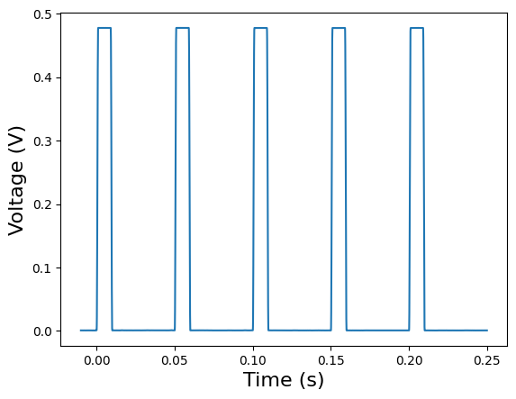
Here, we can see that our stimulus is a square wave with a frequency of 20 Hz and an amplitude of just under 0.5 Volts.
Processing#
There are some relevant pieces of data which are not quite as straightforward to access; some are nested under other attributes. For example, the running speed of the mouse over time is very relevant, but it is nested behind the processing attribute. To see the data structure, we can just use the nwb2widget tool that we showed above in the fifth cell and browse, but here we’ll also show how to read the data manually since the nwb2widget tool can sometimes be slow if there’s a large amount of information in a section.
The processing attribute holds a variety of important pieces of data. processing is a LabelledDict type object like the stimulus templates were. In order to see what the keys are for this LabelledDict, we can just print it and see what attributes we can access:
print(nwbfile_read.processing)
{'behavior': behavior pynwb.base.ProcessingModule at 0x140228458740272
Fields:
  data_interfaces: {
    BehavioralTimeSeries <class 'pynwb.behavior.BehavioralTimeSeries'>
  }
  description: Processed behavioral data
, 'ecephys': ecephys pynwb.base.ProcessingModule at 0x140228460445408
Fields:
  data_interfaces: {
    LFP <class 'pynwb.ecephys.LFP'>
  }
  description: Intermediate data from extracellular electrophysiology recordings, e.g., LFP.
}
As we can see for this example, the keys contained in processing for this mouse are ‘behavior’ and ‘ecephys’. As with the previous sections, it is important to remember that the keys we have here are specific to this optotagging experiment! In general, what information is contained in processing will be experiment-dependent.
Now, let’s access the ‘behavior’ key first to see what it contains:
print(nwbfile_read.processing['behavior'])
behavior pynwb.base.ProcessingModule at 0x140228458740272
Fields:
  data_interfaces: {
    BehavioralTimeSeries <class 'pynwb.behavior.BehavioralTimeSeries'>
  }
  description: Processed behavioral data
Notice here that in order to access a specific key, we simply ask for the name of the key.
Now, when we read this, we can see the ‘behavior’ part of the processing module for this particular experiment contains only one object, data_interfaces. Let’s keep going and see what that contains:
print(nwbfile_read.processing['behavior'].data_interfaces)
{'BehavioralTimeSeries': BehavioralTimeSeries pynwb.behavior.BehavioralTimeSeries at 0x140228458740320
Fields:
  time_series: {
    linear velocity <class 'pynwb.base.TimeSeries'>
  }
}
Notice that to access the subsection of the dictionary key, we call it as an attribute of the key.
In this case the behavior object has one item: the running speed of the mouse during the experiment. This is called the “linear velocity”. In other experiments, we might find the pupil area and/or position here as well.
We can that the linear velocity object by reading through the nested sets printed in our last key. The data_interfaces object possesses a key named BehavioralTimeSeries, which has an attribute time_series inside it. In turn, the attribute time_series possesses the key named linear velocity.
So, the running speed is nested in several layers of LabelledDict type objects. In order to access it, we’ll need to write down the whole “path” to it. Let’s see what information the ‘linear velocity’ key contains.
(For the sake of simplicity, we’ll store the linear velocity data in a different Python object, so that we don’t have to type the full path to the linear velocity every time we wish to examine it.)
running_speed = nwbfile_read.processing['behavior'].data_interfaces['BehavioralTimeSeries'].time_series['linear velocity']
print(running_speed)
linear velocity pynwb.base.TimeSeries at 0x140228458740464
Fields:
  comments: no comments
  conversion: 1.0
  data: <zarr.core.Array '/processing/behavior/BehavioralTimeSeries/linear velocity/data' (624796,) float64 read-only>
  description: The speed of the subject measured over time.
  interval: 1
  offset: 0.0
  resolution: -1.0
  timestamps: <zarr.core.Array '/processing/behavior/BehavioralTimeSeries/linear velocity/timestamps' (624796,) float64 read-only>
  timestamps_unit: seconds
  unit: m/s
This tells us that the ‘linear_velocity’ (which here we’ve stored in running_speed for ease of access) contains several attributes: comments, conversion, data, description, interval, offset, resolution, timestamps, timestamps_unit, and unit. Of these, most are irrelevant for our purposes; the two that contain all the data are:
datacontains the actual velocity at each timestamp.timestampscontains the timestamp for each measurement. These are naturally paired.
We can see that there are 624,796 data points, and that our data is in units of velocity over time. We can access them directly if we want:
print(running_speed.timestamps[:])
print(running_speed.data[:])
[ 454.87926667  454.88925067  454.89926667 ... 6702.80925067 6702.81926667
 6702.82925067]
[ 0.09047513  0.09920467  0.08142761 ... -0.02705582 -0.03619005
 -0.05411164]
And to access a specific data point, we would just use the index in place of the : that tells Python to read all elements of the array.
Now let’s plot the data and time to get an idea of the mouse’s velocity over the course of the experiment:
plt.plot(running_speed.timestamps[:], running_speed.data[:])
plt.xlabel("Time (s)", fontsize=16)
plt.ylabel("Velocity (m/s)", fontsize=16)
plt.show()
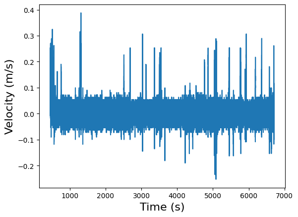
This isn’t the most legible plot, but it’s clear why it isn’t; we have on the order of \(10^5\) measurements, but our time scale is only \(10^3\) s, which means we’re taking around a hundred measurements per second. We can zoom in on a specific time interval to get a better idea of what’s going on in that time interval. We could also apply standard data processing techniques to clean up the signal to improve legibility, but those techniques are beyond the scope of this particular tutorial.
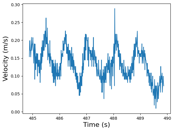
plt.plot(running_speed.timestamps[3000:3500], running_speed.data[3000:3500])
plt.xlabel("Time (s)", fontsize=16)
plt.ylabel("Velocity (m/s)", fontsize=16)
plt.show()
Now let’s back up. There was a second key named ecephys which was contained in the processing attribute of nwbfile_read. Let’s access that and see what data is contained there:
print(nwbfile_read.processing['ecephys'])
ecephys pynwb.base.ProcessingModule at 0x140228460445408
Fields:
  data_interfaces: {
    LFP <class 'pynwb.ecephys.LFP'>
  }
  description: Intermediate data from extracellular electrophysiology recordings, e.g., LFP.
The ecephys object contains one item: the local field potential (LFP) data. LFPs are the signals in the low frequency range (below 500 Hz) that are generated by synchronized synaptic inputs of neuronal populations. This features are known to be correlated with brain and behavioral states. The LFP is computed for each probe independently, so when there are multiple probes, there should be an LFP object for each probe.
In this particular experiment, the path to the LFP data goes through the attribute data_interfaces. Again, for ease of access, we’ll store it in an object so that we don’t have to type out the path every time:
lfp_interface = nwbfile_read.processing['ecephys'].data_interfaces['LFP']
print(lfp_interface)
LFP pynwb.ecephys.LFP at 0x140228458739984
Fields:
  electrical_series: {
    ElectricalSeriesProbeA-LFP <class 'pynwb.ecephys.ElectricalSeries'>,
    ElectricalSeriesProbeB-LFP <class 'pynwb.ecephys.ElectricalSeries'>
  }
Looking at the contents of the LFP data, we have two probes listed. As expected, each one of them contains LFP data. Let’s take a look at one of them to start:
lfp_es = lfp_interface.electrical_series['ElectricalSeriesProbeA-LFP']
print(lfp_es)
ElectricalSeriesProbeA-LFP pynwb.ecephys.ElectricalSeries at 0x140228460444496
Fields:
  comments: no comments
  conversion: 4.679999828338622e-06
  data: <zarr.core.Array '/processing/ecephys/LFP/ElectricalSeriesProbeA-LFP/data' (15650092, 384) int16 read-only>
  description: LFP voltage traces from ProbeA
  electrodes: electrodes <class 'hdmf.common.table.DynamicTableRegion'>
  offset: 0.0
  rate: 2500.0
  resolution: -1.0
  starting_time: 447.9456
  starting_time_unit: seconds
  unit: volts
Reading off the information about the data recorded by Probe A, we can see that we only have one set of data here. There, we have 15,661,294 data points for each of the 384 channels on the Neuropixels probe. None of this data is directly associated with a time coordinate. Instead, we’re told the sampling rate of 2500 Hz and the starting time. Thus, if we want to plot this, we’ll have to construct the timestamps manually by taking the starting time and then appending times at 1/2500 s intervals until we have 15,661,294 timestamps.
Fortunately, this is a task computers excel at:
lfp_num_samples = lfp_es.data.shape[0]
lfp_timestamps = lfp_es.starting_time + np.arange(lfp_num_samples) / lfp_es.rate
Next we can examine what’s contained in the data. Here, we’ll pick a specific interval instead of plotting for the entire experiment to enhance legibility. (As with the previous section, we would still need to do a significant amount of signal processing to analyze this data).
plt.imshow(lfp_es.data[50000:60000,0:350].T, origin='lower', aspect='auto')
plt.ylabel('Channel')
plt.xlabel('Sample')
Text(0.5, 0, 'Sample')
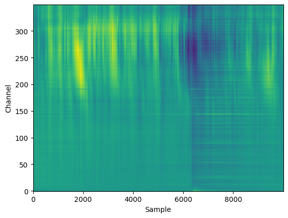
Here, we are not plotting channels above 350, as they were outside of the brain and thus did not have meaningful data. In this time period, we can see some clear oscillatory activity in channels 200-350, which were likely in the cortex.
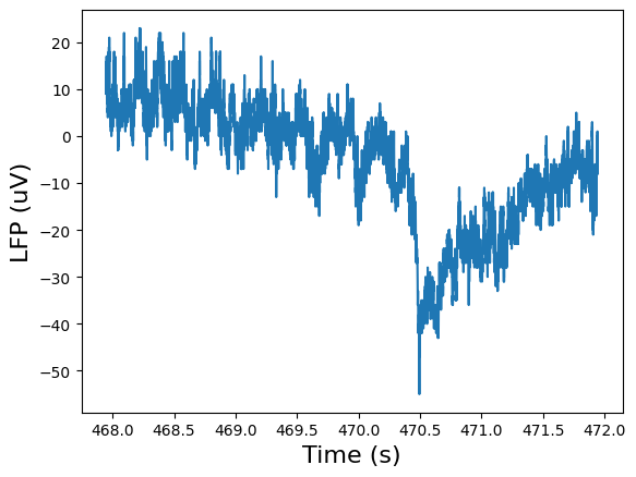
Instead of looking at all 384 channels, we can also examine just a single channel, and we can plot it against time to see what the LFP looked like for that channel.
channel = 99
raw_data = lfp_es.data[:, channel]

print(raw_data.shape)

plt.plot(lfp_timestamps[50000:60000], raw_data[50000:60000])
plt.xlabel("Time (s)", fontsize=16)
plt.ylabel("LFP (uV)", fontsize=16)
plt.show()
(15650092,)
Finally, we can also examine the information contained in the electrodes attribute of the probe we’re investigating:
print(lfp_es.electrodes.shape)
(384, 10)
Here, we can see that we have ten entries for every channel.
The NWB file contains other data as well which can be explored using the methods we’ve detailed in this tutorial; we will not detail every piece of accessible information here, but hopefully it should be clear from these examples how one can navigate and extract data from an NWB file. Once finished, we should then close the NWB file.
io.close()