Visual Coding Ophys Dataset

import pandas as pd 
import numpy as np
from datetime import datetime, date

from aind_data_access_api.document_db import MetadataDbClient

API_GATEWAY_HOST = "api.allenneuraldynamics.org"
DATABASE = 'metadata_index'
COLLECTION = 'data_assets'

docdb_api_client = MetadataDbClient(
   host=API_GATEWAY_HOST,
    version="v2",
   database=DATABASE,
   collection=COLLECTION,
)
print(docdb_api_client._base_url)

https://api.allenneuraldynamics.org/v2/metadata_index/data_assets

Dataset

We will start exploring the parameters of the dataset to learn what data is available. We can query the database and create a dataframe of some of the key metadata fields:

aggregate = [
  {
    "$match": {
      "data_description.project_name": {
        "$regex": "Allen Brain Observatory - Visual Coding Ophys",
        "$options": "i"
      },
    }
  },
  {
    "$project": {
      "name": 1, 
      "subject_id": "$data_description.subject_id",
      "genotype": "$subject.subject_details.genotype", 
      "date_of_birth": "$subject.subject_details.date_of_birth", 
      "sex": "$subject.subject_details.sex", 
      "session_time": "$acquisition.acquisition_start_time",
      "project_name": "$data_description.project_name", 
      "modality": "$data_description.modalities.name",
      "depth": "$acquisition.data_streams.configurations.images.planes.depth",
      "targeted_structure": "$acquisition.data_streams.configurations.images.planes.targeted_structure.acronym",
      "session_type": "$acquisition.acquisition_type",
      "container_id": { "$arrayElemAt": ["$data_description.tags", 2] },
    }
  },
]
    
records = docdb_api_client.aggregate_docdb_records(
    pipeline = aggregate,
)

df = pd.DataFrame(records)

df['session_date'] = df.apply(lambda x: datetime.fromisoformat(x['session_time']).date(), axis=1)
df['session_time'] = df.apply(lambda x: datetime.fromisoformat(x['session_time']).time(), axis=1)
df['date_of_birth'] = df.apply(lambda x: datetime.strptime(x['date_of_birth'], '%Y-%m-%d').date(), axis=1)
df['age'] = df.apply(lambda x: (x['session_date'] - x['date_of_birth']).days, axis=1)

df['depth'] = df.apply(lambda x: list(np.array(x['depth']).flatten())[0], axis=1)
df['targeted_structure'] = df.apply(lambda x: str(np.array(x['targeted_structure']).flatten()[0]), axis=1)

df['container_id'] = df.apply(lambda x: int(x['container_id'].split(' ')[-1]), axis=1)

order = ['project_name','_id','name','subject_id','genotype','date_of_birth','sex','modality',
         'session_type','session_date','age','session_time','depth', 'targeted_structure','container_id']
df = df[order]

df.head()

	project_name	_id	name	subject_id	genotype	date_of_birth	sex	modality	session_type	session_date	age	session_time	depth	targeted_structure	container_id
0	Allen Brain Observatory - Visual Coding Ophys	c88f22d2-a6a5-42a8-805a-80869635cfba	261967_2016-11-08_11-29-45_nwb_2026-08-19_17-4...	261967	Nr5a1-Cre/wt;Camk2a-tTA/wt;Ai93(TITL-GCaMP6f)/wt	2016-06-13	Female	[Behavior videos, Planar optical physiology]	three_session_B	2016-11-08	148	11:29:45	350	VISpm	555749366
1	Allen Brain Observatory - Visual Coding Ophys	ae362a40-f97b-495e-96ec-fea98b19d753	280643_2016-12-22_11-09-41_nwb_2026-08-19_17-1...	280643	Emx1-IRES-Cre/wt;Camk2a-tTA/wt;Ai93(TITL-GCaMP...	2016-09-17	Male	[Planar optical physiology, Behavior videos]	three_session_B	2016-12-22	96	11:09:41	175	VISal	560876149
2	Allen Brain Observatory - Visual Coding Ophys	f1335249-f136-4b7b-a9f2-6b2b920d8c25	229105_2016-03-09_11-13-50_nwb_2026-08-19_18-1...	229105	Cux2-CreERT2/Cux2-CreERT2;Camk2a-tTA/wt;Ai93(T...	2015-12-14	Male	[Planar optical physiology, Behavior videos]	three_session_C	2016-03-09	86	11:13:50	175	VISal	511510998
3	Allen Brain Observatory - Visual Coding Ophys	e556a3a4-edba-423e-a0eb-f239bf42e6cd	361635_2018-02-19_11-00-16_nwb_2026-08-19_18-1...	361635	Slc17a7-IRES2-Cre/wt;Camk2a-tTA/wt;Ai93(TITL-G...	2017-10-12	Female	[Planar optical physiology, Behavior videos]	three_session_A	2018-02-19	130	11:00:16	375	VISpm	665413463
4	Allen Brain Observatory - Visual Coding Ophys	8a249c0b-ce8e-4b28-804b-e05755280db2	336246_2017-08-30_11-08-01_nwb_2026-08-19_17-2...	336246	Vip-IRES-Cre/wt;Ai148(TIT2L-GC6f-ICL-tTA2)/wt	2017-06-03	Female	[Planar optical physiology, Behavior videos]	three_session_A	2017-08-30	88	11:08:01	275	VISl	614556104

Targeted structures

What brain regions were recorded across the dataset? Look at the unique targeted structures

df.targeted_structure.unique().tolist()

['VISpm', 'VISal', 'VISl', 'VISp', 'VISrl', 'VISam']

We see that data was collected in six different visual areas. VISp is the primary visual cortex, also known as V1. The others are higher visual areas (HVAs) that surround VISp. You can learn more about these areas and how we map them here.

Cre lines and reporters

We used Cre lines to drive the expression of GCaMP6 in specific populations of neurons. We also use four different reporter lines for GCaMP6. The identity of both the driver and the reporter are contained within the genotype of the mouse. The genotype also conveys whether a given subject is homozygous or heterozygous (i.e. whether the subject has one or two copies of any element). So far, we see no significant differences between homozygous and heterozygous mice, and we recommend analyzing them together. But as a result, a list of unique genotypes is over complete

We can find a list of all the cre lines used in this dataset as follows

cre_lines = []
for item in df.genotype.unique():
    cre_lines.append(item.split('/')[0])
cre_lines = np.unique(cre_lines)
cre_lines.tolist()

['Cux2-CreERT2',
 'Emx1-IRES-Cre',
 'Fezf2-CreER',
 'Nr5a1-Cre',
 'Ntsr1-Cre_GN220',
 'Pvalb-IRES-Cre',
 'Rbp4-Cre_KL100',
 'Rorb-IRES2-Cre',
 'Scnn1a-Tg3-Cre',
 'Slc17a7-IRES2-Cre',
 'Sst-IRES-Cre',
 'Tlx3-Cre_PL56',
 'Vip-IRES-Cre']

See Transgenic tools to learn more about these Cre lines and reporters.

Note

Reporter lines: All the experiments in this dataset use GCaMP6. The large majority use GCaMP6f and only a few use GCaMP6s. However, you see four different reporters listed here. Why is this? Ai93 is the GCaMP6f reporter we used with the excitatory Cre lines. However, this reporter does not work well for inhibitory Cre lines. We used Ai148, another GCaMP6f reporter, with Vip-IRES-Cre and Sst-IRES-Cre. However, this didn’t work with the Pvalb-IRES-Cre. We use Ai162, a GCaMP6s reporter with Pvalb. Additionally, to have a GCaMP6f vs GCaMP6s comparison, we collected a small number of experiments using Ai94 with the Slc17a7-IRES2-Cre. This is a GCaMP6s reporter that complements Ai93. Slc17a7-IRES2-Cre is the only Cre line that was recorded using multiple reporter types.

Imaging depths

Each experiment was collected at a single imaging depth.

df.depth.unique().tolist()

[350,
 175,
 375,
 275,
 300,
 276,
 550,
 625,
 285,
 250,
 400,
 390,
 265,
 325,
 320,
 335,
 185,
 570,
 205,
 365,
 435,
 225,
 200,
 195]

These values are in µm below the surface of the cortex. This is a long list and some of the values don’t differ by very much. How meaningful is it? We roughly consider depths less than 250 to be layer 2/3, 250-350 to be layer 4, 350-500 to be layer 5, and over 500 to be layer 6. Keep in mind, much of the imaging here was done with layer specific Cre lines, so for most purposes the best way to get layer specificity is to select appropriate Cre lines.

Experiment containers & sessions

The experiment {term} container describes a set of 3 imaging sessions performed for the same field of view (ie. same targeted structure and imaging depth in the same mouse that targets the same set of neurons). Each experiment container has a unique ID number.

Let’s look at all of the sessions in one experiment container

df[df.container_id==df.container_id[0]]

	project_name	_id	name	subject_id	genotype	date_of_birth	sex	modality	session_type	session_date	age	session_time	depth	targeted_structure	container_id
0	Allen Brain Observatory - Visual Coding Ophys	c88f22d2-a6a5-42a8-805a-80869635cfba	261967_2016-11-08_11-29-45_nwb_2026-08-19_17-4...	261967	Nr5a1-Cre/wt;Camk2a-tTA/wt;Ai93(TITL-GCaMP6f)/wt	2016-06-13	Female	[Behavior videos, Planar optical physiology]	three_session_B	2016-11-08	148	11:29:45	350	VISpm	555749366
174	Allen Brain Observatory - Visual Coding Ophys	4f8a2bc2-b805-463c-a8b4-f2cdb2d3ccd6	261967_2016-11-03_11-24-50_nwb_2026-08-19_17-5...	261967	Nr5a1-Cre/wt;Camk2a-tTA/wt;Ai93(TITL-GCaMP6f)/wt	2016-06-13	Female	[Planar optical physiology, Behavior videos]	three_session_A	2016-11-03	143	11:24:50	350	VISpm	555749366
1277	Allen Brain Observatory - Visual Coding Ophys	f90f0f7c-c149-454e-9817-7b480d3e832a	261967_2016-11-10_11-06-49_nwb_2026-08-19_17-5...	261967	Nr5a1-Cre/wt;Camk2a-tTA/wt;Ai93(TITL-GCaMP6f)/wt	2016-06-13	Female	[Behavior videos, Planar optical physiology]	three_session_C2	2016-11-10	150	11:06:49	350	VISpm	555749366

Notice that the subject_id, genotype, targeted structure, depth are all the same. What differs are the session_type, the session_date, and age.

Each session_type has a different set of visual stimuli.

As you see, each experiment container has three different session types. For the data published in June 2016 and October 2016, the last session is three_session_C</b<> while the data published after this were collected using three_session_C2. The key difference between these sessions is a change in the locally sparse noise stimulus. This is described more here.

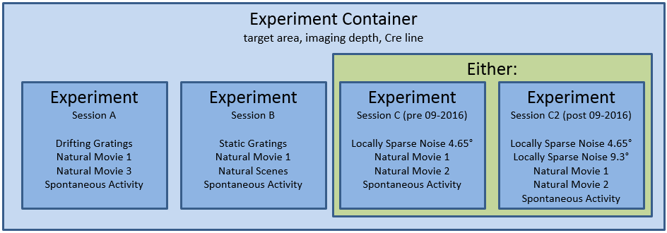
Exercise: How many sessions were collected in each cortical visual area for each Cre line?

# we made a list of cre_lines above
areas = df.targeted_structure.unique().tolist() #list of areas

df2 = pd.DataFrame(columns=areas, index=cre_lines)
for cre in cre_lines:
  for area in areas:
    df2.loc[cre, area] = len(df[(df.targeted_structure==area)&(df['genotype'].str.contains(cre))])
df2

	VISpm	VISal	VISl	VISp	VISrl	VISam
Cux2-CreERT2	51	39	45	63	36	33
Emx1-IRES-Cre	12	21	24	60	27	9
Fezf2-CreER	0	0	15	12	0	0
Nr5a1-Cre	21	24	24	36	21	21
Ntsr1-Cre_GN220	15	0	21	18	0	0
Pvalb-IRES-Cre	0	0	15	48	0	0
Rbp4-Cre_KL100	21	24	27	33	12	27
Rorb-IRES2-Cre	27	21	21	33	15	24
Scnn1a-Tg3-Cre	0	0	0	27	0	0
Slc17a7-IRES2-Cre	45	6	48	60	6	6
Sst-IRES-Cre	42	3	45	51	6	0
Tlx3-Cre_PL56	0	0	9	18	0	0
Vip-IRES-Cre	48	0	51	51	0	0