
Visual Behavior Ophys Experiment Data#
Below we we will learn how to load optical physiology and behavior data for one imaging plane from a Visual Behavior Ophys session using the AllenSDK. It describes the type of data available and shows a few simple ways of plotting calcium fluorescence traces along with the animal’s behavior and stimulus presentation times.
We need to import libraries for plotting and manipulating data:
import numpy as np
import pandas as pd
import seaborn as sns
import matplotlib.pyplot as plt

%matplotlib notebook
%matplotlib inline
# Import allenSDK and check the version, which should be 2.16.2
import allensdk
allensdk.__version__
'2.16.2'
Load the cache and get metadata tables#
# import the behavior ophys project cache class from SDK to be able to load the data
from allensdk.brain_observatory.behavior.behavior_project_cache import VisualBehaviorOphysProjectCache
/opt/envs/allensdk/lib/python3.10/site-packages/tqdm/auto.py:21: TqdmWarning: IProgress not found. Please update jupyter and ipywidgets. See https://ipywidgets.readthedocs.io/en/stable/user_install.html
  from .autonotebook import tqdm as notebook_tqdm
# Set the path to the dataset
cache_dir = '/root/capsule/data/'
# If you are working with data in the cloud in Code Ocean,
# or if you have already downloaded the full dataset to your local machine,
# you can instantiate a local cache
cache = VisualBehaviorOphysProjectCache.from_local_cache(cache_dir=cache_dir, use_static_cache=True)

# If you are working with the data locally for the first time, you need to instantiate the cache from S3:
# cache = VisualBehaviorOphysProjectCache.from_s3_cache(cache_dir=cache_dir)
/opt/envs/allensdk/lib/python3.10/site-packages/allensdk/brain_observatory/behavior/behavior_project_cache/behavior_project_cache.py:135: UpdatedStimulusPresentationTableWarning:
	As of AllenSDK version 2.16.0, the latest Visual Behavior Ophys data has been significantly updated from previous releases. Specifically the user will need to update all processing of the stimulus_presentations tables. These tables now include multiple stimulus types delineated by the columns `stimulus_block` and `stimulus_block_name`.

The data that was available in previous releases are stored in the block name containing 'change_detection' and can be accessed in the pandas table by using:
	`stimulus_presentations[stimulus_presentations.stimulus_block_name.str.contains('change_detection')]`
  warnings.warn(
# get metadata tables
behavior_session_table = cache.get_behavior_session_table()
ophys_session_table = cache.get_ophys_session_table()
ophys_experiment_table = cache.get_ophys_experiment_table()

#print number of items in each table for all imaging and behavioral sessions
print('Number of behavior sessions = {}'.format(len(behavior_session_table)))
print('Number of ophys sessions = {}'.format(len(ophys_session_table)))
print('Number of ophys experiments = {}'.format(len(ophys_experiment_table)))
Number of behavior sessions = 4782
Number of ophys sessions = 703
Number of ophys experiments = 1936
The term ophys experiment is used to describe one imaging plane during one ophys session. Each ophys session can contain one or more ophys experiments (imaging planes) depending on which microscope was used.
For datasets acquired using a single-plane imaging microscope (equipment_name = CAMP#.#), there will be only 1 ophys_experiment_id per ophys_session_id. For sessions acquired with the multi-plane Mesoscope (equipment_name = MESO.#), there can be up to 8 ophys experiments (i.e. imaging planes) associated with that session.
The ophys_session_table contains metadata for each imaging session and is organized by the ophys_session_id.
The ophys_experiment_table contains metadata for each imaging plane in each session and is organized by the ophys_experiment_id. This table includes all the metadata provided by the ophys_session_table, as well as information specific to the imaging plane, such as the imaging_depth and targeted_structure.
A single imaging plane (aka ophys experiment) is linked across sessions using the ophys_container_id. An ophys container can contain a variable number of ophys_experiment_ids depending on which session_types were acquired for that imaging plane, and which passed quality control checks.
The behavior_session_table contains metadata related to the full training history of each mouse and is organized by the behavior_session_id. Some behavior sessions took place under the 2-photon microscope (session_type beginning with OPHYS_) and will have an associated ophys_session_id if the ophys data passed quality control and is available for analysis.
Some ophys sessions may not pass quality control, but the behavior data is still provided in the behavior_session_table. These sessions will have a session_type beginning with OPHYS_ but will not have an associated ophys_session_id.
In this notebook, we will use the ophys_experiment_table to select experiments of interest and look at them in a greater detail.
Filter the ophys_experiment_table to identify experiments of interest#
# let's print a sample of 5 rows to see what's in the table
ophys_experiment_table.sample(5)
| behavior_session_id | ophys_session_id | ophys_container_id | mouse_id | indicator | full_genotype | driver_line | cre_line | reporter_line | sex | ... | passive | experience_level | prior_exposures_to_session_type | prior_exposures_to_image_set | prior_exposures_to_omissions | date_of_acquisition | equipment_name | published_at | isi_experiment_id | file_id | |
|---|---|---|---|---|---|---|---|---|---|---|---|---|---|---|---|---|---|---|---|---|---|
| ophys_experiment_id | |||||||||||||||||||||
| 877669822 | 873517635 | 873247524 | 1018027608 | 449653 | GCaMP6f | Vip-IRES-Cre/wt;Ai148(TIT2L-GC6f-ICL-tTA2)/wt | [Vip-IRES-Cre] | Vip-IRES-Cre | Ai148(TIT2L-GC6f-ICL-tTA2) | M | ... | False | Novel 1 | 0 | 0 | 3 | 2019-05-22 09:12:30.484000+00:00 | MESO.1 | 2021-03-25 | 846102910 | 1204 |
| 1059963010 | 1059890582 | 1059871455 | 1058209392 | 539518 | GCaMP6f | Slc17a7-IRES2-Cre/wt;Camk2a-tTA/wt;Ai93(TITL-G... | [Slc17a7-IRES2-Cre, Camk2a-tTA] | Slc17a7-IRES2-Cre | Ai93(TITL-GCaMP6f) | F | ... | False | Familiar | 0 | 11 | 2 | 2020-10-29 10:34:15.526000+00:00 | CAM2P.4 | 2021-03-25 | 1047947399 | 832 |
| 853362777 | 853266283 | 853177377 | 1018027868 | 438912 | GCaMP6f | Vip-IRES-Cre/wt;Ai148(TIT2L-GC6f-ICL-tTA2)/wt | [Vip-IRES-Cre] | Vip-IRES-Cre | Ai148(TIT2L-GC6f-ICL-tTA2) | M | ... | True | Novel >1 | 0 | 2 | 6 | 2019-04-17 14:01:59.667000+00:00 | MESO.1 | 2021-03-25 | 817613066 | 775 |
| 945473009 | 944950609 | 944810835 | 929913236 | 468866 | GCaMP6f | Vip-IRES-Cre/wt;Ai148(TIT2L-GC6f-ICL-tTA2)/wt | [Vip-IRES-Cre] | Vip-IRES-Cre | Ai148(TIT2L-GC6f-ICL-tTA2) | F | ... | False | Familiar | 0 | 20 | 6 | 2019-09-12 10:57:08.386000+00:00 | CAM2P.4 | 2021-03-25 | 885422294 | 1835 |
| 1101564165 | 1101486792 | 1101470236 | 1099411361 | 555970 | GCaMP6f | Sst-IRES-Cre/wt;Ai148(TIT2L-GC6f-ICL-tTA2)/wt | [Sst-IRES-Cre] | Sst-IRES-Cre | Ai148(TIT2L-GC6f-ICL-tTA2) | M | ... | True | Familiar | 0 | 39 | 3 | 2021-05-06 12:51:06.356000+00:00 | MESO.1 | 2021-08-12 | 1074688680 | 387 |
5 rows × 30 columns
You can get ophys_experiment_ids corresponding to specific experimental conditions by filtering the table using the columns. Here, we can select experiments from mice from the Sst-IRES-Cre Driver Line, also called a {term}’Cre line’, as well as filter by session_number to identify experiments from the first session with the novel images, which always has a session_type starting with OPHYS_4, and can be identified using the abbreviated session_number column which is agnostic to which specific image set was used). You can use the prior_exposures_to_image_set column to ensure that the session was truly the first day with the novel image set, and not a retake of the same session_type.
# get all Sst experiments for ophys session 4
selected_experiment_table = ophys_experiment_table[(ophys_experiment_table.cre_line=='Sst-IRES-Cre')&
                        (ophys_experiment_table.session_number==4) &
                        (ophys_experiment_table.prior_exposures_to_image_set==0)]
print('Number of experiments: {}'.format(len(selected_experiment_table)))
Number of experiments: 58
Remember that any given experiment (defined by its ophys_experiment_id) contains data from only one imaging plane, in one session. There can be multiple experiments (imaging planes) recorded in the same imaging session if the multi-plane 2-photon microscope was used, but there can never be multiple sessions for a given ophys_experiment_id.
Here, we can check how many unique imaging sessions are associated with experiments selected above.
print('Number of unique sessions: {}'.format(len(selected_experiment_table['ophys_session_id'].unique())))
Number of unique sessions: 19
Load data for one experiment#
Let’s pick an experiment from the table and plot example ophys and behavioral data.
# select first experiment from the table to look at in more detail.
ophys_experiment_id = selected_experiment_table.index[0]

# load the data for this ophys experiment from the cache
ophys_experiment = cache.get_behavior_ophys_experiment(ophys_experiment_id)
/opt/envs/allensdk/lib/python3.10/site-packages/hdmf/utils.py:668: UserWarning: Ignoring cached namespace 'core' version 2.6.0-alpha because version 2.7.0 is already loaded.
  return func(args[0], **pargs)
The get_behavior_ophys_experiment() method returns a python object containing all data and metadata for the provided ophys_experiment_id.
What are the attributes of the ophys_experiment object?
# Get all attributes & methods
attributes = ophys_experiment.list_data_attributes_and_methods()
# Let's focus on attributes for now, remove the methods, which start with "get"
[attribute for attribute in attributes if 'get' not in attribute]
['average_projection',
 'behavior_session_id',
 'cell_specimen_table',
 'corrected_fluorescence_traces',
 'demixed_traces',
 'dff_traces',
 'events',
 'eye_tracking',
 'eye_tracking_rig_geometry',
 'licks',
 'max_projection',
 'metadata',
 'motion_correction',
 'neuropil_traces',
 'ophys_experiment_id',
 'ophys_session_id',
 'ophys_timestamps',
 'raw_running_speed',
 'rewards',
 'roi_masks',
 'running_speed',
 'segmentation_mask_image',
 'stimulus_presentations',
 'stimulus_templates',
 'stimulus_timestamps',
 'task_parameters',
 'trials']
Note that any attribute can be followed by a ? in a Jupyter Notebook to see the docstring. For example, running the cell below will make a frame appear at the bottom of your browser with the docstring for the metadata attribute.
ophys_experiment.metadata?
Experiment metadata#
Get the metadata for this experiment using the metadata attribute of the OphysExperiment class.
ophys_experiment.metadata
{'equipment_name': 'MESO.1',
 'sex': 'F',
 'age_in_days': 213,
 'stimulus_frame_rate': 60.0,
 'session_type': 'OPHYS_4_images_B',
 'date_of_acquisition': datetime.datetime(2019, 9, 27, 8, 58, 37, 5000, tzinfo=tzutc()),
 'reporter_line': 'Ai148(TIT2L-GC6f-ICL-tTA2)',
 'cre_line': 'Sst-IRES-Cre',
 'behavior_session_uuid': UUID('40897cd4-3279-4a2d-b65d-b3f984e34e17'),
 'driver_line': ['Sst-IRES-Cre'],
 'mouse_id': '457841',
 'project_code': 'VisualBehaviorMultiscope',
 'full_genotype': 'Sst-IRES-Cre/wt;Ai148(TIT2L-GC6f-ICL-tTA2)/wt',
 'behavior_session_id': 957032492,
 'indicator': 'GCaMP6f',
 'emission_lambda': 520.0,
 'excitation_lambda': 910.0,
 'ophys_container_id': 1018028342,
 'field_of_view_height': 512,
 'field_of_view_width': 512,
 'imaging_depth': 150,
 'targeted_imaging_depth': 150,
 'imaging_plane_group': 0,
 'imaging_plane_group_count': 4,
 'ophys_experiment_id': 957759562,
 'ophys_frame_rate': 11.0,
 'ophys_session_id': 957020350,
 'targeted_structure': 'VISp'}
Here you can see that this experiment was in Sst Cre line, in a female mouse at 233 days old, recorded using mesoscope, at an imaging depth of 150 microns, in primary visual cortex (VISp). This experiment is also from OPHYS 1 session using image set A.
- age_in_days
(int) age of mouse in days
- behavior_session_id
(int) unique identifier for a behavior session
- behavior_session_uuid
(uuid) unique identifier for a behavior session
- cre_line
(string) cre driver line for a transgenic mouse
- date_of_acquisition
(date time object) date and time of experiment acquisition, yyyy-mm-dd hh:mm:ss.
- driver_line
(list of string) all driver lines for transgenic mouse
emission_lambda: (float) wavelength (in nanometers) the 2 photon microscope is tuned to based on transgenic reporter line
- equipment_name
(string) identifier for equipment data was collected on
- excitation_lambda
(float 64) wavelength (in nanometers) of the two photon laser
- field_of_view_height
(int) field of view height in pixels
- field_of_view_width
(int) field of view width in pixels
- full_genotype
(string) full genotype of transgenic mouse
- imaging_depth
(int) depth in microns from the cortical surface, where the data was collected
- imaging_plane_group
(none or int) a grouping number assigned to paired planes (experiments) that were simultaneously recorded, applies to mesoscope sessions only
- imaging_plane_group_count
(int) total number of imaging plane groups for a mesoscope session
- mouse_id
(int) unique identifier for a mouse
- ophys_container_id
(int) unique identifier for a container, which connects all sessions acquired for a given ophys field of view
- ophys_experiment_id
(int) unique identifier for an ophys experiment, corresponding to one imaging plane in one recording session
- ophys_frame_rate
(float 64) rate (in Hz) that the two photon microscope collected frames for an individual imaging plane / field of view
- ophys_session_id
(int) unique identifier for a ophys session
- project_code
(str) name of the cohort the mouse belonged two; each cohort used a unique stimulus set and imaging configuration
- reporter_line
(string) reporter line for transgenic mouse
- session_type
(string) visual stimulus type displayed during behavior session
- sex
(string) sex of the mouse
- stimulus_frame_rate
(float) frame rate (Hz) at which the visual stimulus is displayed
- targeted_imaging_depth
(int) target depth within the cortex where the data was intended to be collected
- targeted_structure
(string) brain area targeted for the imaging plane in this experiment
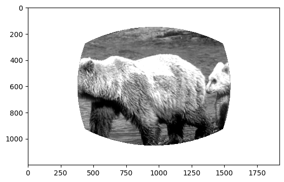
Max projection image#
Plot the maximum intensity projection image for this imaging plane.
plt.imshow(ophys_experiment.max_projection, cmap='gray')
<matplotlib.image.AxesImage at 0x7fb4773da680>
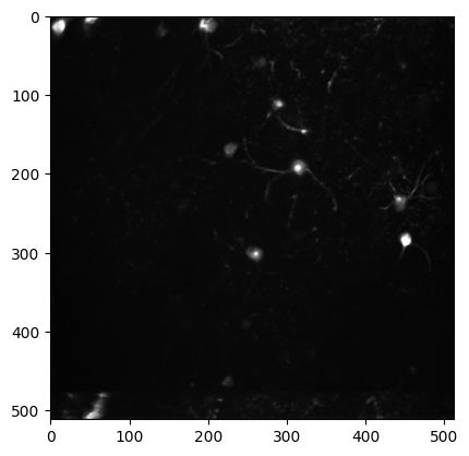
The max_projection is a 2D image of the maximum intensity value for each pixel across the entire 2-photon movie recorded during an imaging session. Plotting the max projection can give you a sense of how many neurons were visible during imaging and how clear and stable the imaging session was.
Average projection#
Plot the average projection image for this imaging plane.
plt.imshow(ophys_experiment.average_projection, cmap='gray')
<matplotlib.image.AxesImage at 0x7fb514adae60>
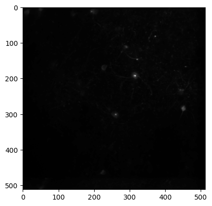
The average_projection is a2D image of the microscope field of view, averaged across the session.
Cell specimen table#
Examine the cell_specimen_table which contains metadata about each segmented neuron.
ophys_experiment.cell_specimen_table.sample(3)
| cell_roi_id | height | mask_image_plane | max_correction_down | max_correction_left | max_correction_right | max_correction_up | valid_roi | width | x | y | roi_mask | |
|---|---|---|---|---|---|---|---|---|---|---|---|---|
| cell_specimen_id | ||||||||||||
| 1086615620 | 1080740955 | 17 | 0 | 5.0 | 25.0 | 3.0 | 30.0 | True | 19 | 280 | 104 | [[False, False, False, False, False, False, Fa... |
| 1086616398 | 1080740952 | 20 | 0 | 5.0 | 25.0 | 3.0 | 30.0 | True | 19 | 220 | 161 | [[False, False, False, False, False, False, Fa... |
| 1086614819 | 1080740886 | 22 | 0 | 5.0 | 25.0 | 3.0 | 30.0 | True | 16 | 443 | 275 | [[False, False, False, False, False, False, Fa... |
- cell_specimen_id [index]
(int) unified id of segmented cell across experiments (assigned after cell matching)
- cell_roi_id
(int) experiment specific id of segmented roi (assigned before cell matching)
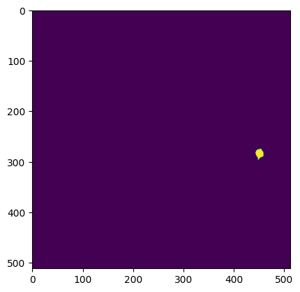
- roi_mask
(array of bool) an image array that displays the location of the roi mask in the field of view
- valid_roi
(bool) indicates if cell classification found the segmented ROI to be a cell or not (True = cell, False = not cell). Only valid cells are provided in the released dataset.
- width
(int) width of ROI in pixels
- height
(int) height of ROI/cell in pixels
- x
(float) x position of ROI in field of view in pixels (top left corner)
- y
(float) y position of ROI in field of view in pixels (top left corner)
- mask_image_plane
(int) which image plane an ROI resides on. Overlapping ROIs are stored on different mask image planes
- max_correction_down
(float) max motion correction in down direction in pixels
- max_correction_left
(float) max motion correction in left direction in pixels
- max_correction_right
(float) max motion correction in right direction in pixels
- max_correction_up
(float) max motion correction in up direction in pixels
What do the ROI masks look like?
# plot one ROI mask
plt.imshow(ophys_experiment.cell_specimen_table.iloc[1]['roi_mask'])
<matplotlib.image.AxesImage at 0x7fb4760c7e20>
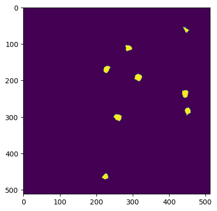
Segmentation mask image#
A 2D image of all segmented ROIs can be viewed using the segmentation_mask_image attribute.
segmentation_mask_image
plt.imshow(ophys_experiment.segmentation_mask_image)
<matplotlib.image.AxesImage at 0x7fb477283a00>
Cell activity traces#
There are several versions of cell activity traces, corresponding to different stages of the data processing pipeline.
cell activity traces recorded on the single-plane Scientifica microscopes are sampled at 30Hz, while cell activity recorded on the multi-plane Mesoscope are recorded at 11Hz
After ROIs are segmented, the average fluorescence value within the ROI is computed for each frame of the 2-photon movie, resulting in a trace of raw fluorescence over time, in arbitrary units. A fluorescence trace for the region surrounding the ROI, containing neuropil and other cell bodies, is computed and subtracted from the raw fluorescence of the cell to remove contamination from surrounding pixels. If two ROIs are overlapping with each other, they are demixed to ensure that the fluorescence signal is attributed to the correct ROI.
The neuropil corrected, demixed traces, called corrected_fluorescence_traces are then baseline subtracted and normalized to produce dff_traces which provide a fractional change in fluorescence over time relative to the ROI’s baseline fluorescence. These are the cell activity traces that are typically used for analysis.
Finally, an event detection algorithm is run on the dff_traces to determine the time and magnitude of calcium events and reduce potential confounds arising from features of the calcium indicator. More specifically, the binding kinetics of the calcium indicator GCaMP6 result in a fast rise in fluorescence following spiking activity, but a much slower decay time. This slow decay of the calcium signal can cause problems some types of analysis because repeated bursts of action potentials can cause the calcium signal to summate, resulting in a magnitude that is no longer proportional to the cell’s activity. The deconvolved events remove contamination due to this slow decay, and are useful in cases where timing precision is particularly important.
The dataframes provided for dff_traces, events, corrected_fluorescence_traces, demixed_traces, and neuropil_traces all share the same index, the cell_specimen_id and one column, the cell_roi_id.
- cell_specimen_id [index]
(int) unified ID of segmented cell across experiments (assigned after cell matching)
- cell_roi_id
(int) experiment specific ID of segmented cell (assigned before cell matching)
The unique columns of the two most important types of traces, dff_traces and events are described below.
dF/F traces#
Examine dff_traces for the first 10 cells this experiment.
ophys_experiment.dff_traces.head(10)
| cell_roi_id | dff | |
|---|---|---|
| cell_specimen_id | ||
| 1086614149 | 1080740882 | [0.3417784869670868, 0.1917504370212555, 0.169... |
| 1086614819 | 1080740886 | [0.0, -2.010002374649048, -1.3567286729812622,... |
| 1086614512 | 1080740888 | [0.07121878117322922, 0.10929209738969803, 0.0... |
| 1086613265 | 1080740947 | [0.3090711534023285, 0.02156120352447033, -0.0... |
| 1086616398 | 1080740952 | [0.0, 0.15438319742679596, 0.37885594367980957... |
| 1086615620 | 1080740955 | [0.15867245197296143, 0.15752384066581726, 0.2... |
| 1086615201 | 1080740967 | [0.42869994044303894, 0.23723232746124268, -0.... |
| 1086616101 | 1080741008 | [0.727859377861023, 0.20604123175144196, 0.333... |
- dff
(list of float) fractional fluorescence values relative to baseline (arbitrary units). Each value corresponds to one frame of the 2-photon movie.
If you don’t want dff in a pandas dataframe format, you can convert dff_traces to an array, using the np.vstack function.
dff_array = np.vstack(ophys_experiment.dff_traces.dff.values)
print('This array contains dff traces from {} neurons and it is {} samples long.'.format(dff_array.shape[0], dff_array.shape[1]))
This array contains dff traces from 8 neurons and it is 48284 samples long.
Events#
events are computed for each cell as described in Giovannucci et al. 2019. The magnitude of events approximates the firing rate of neurons with the resolution of about 200 ms. The biggest advantage of using events over dff traces is they exclude prolonged calcium transients that may contaminate neural responses to subsequent stimuli. You can also use filtered_events which are events convolved with a filter created using stats.halfnorm method to generate a more continuous trace of activity.
Examine events for the first 10 cells this experiment.
ophys_experiment.events.head(10)
| cell_roi_id | events | filtered_events | lambda | noise_std | |
|---|---|---|---|---|---|
| cell_specimen_id | |||||
| 1086614149 | 1080740882 | [0.0, 0.0, 0.0, 0.0, 0.0, 0.0, 0.0, 0.0, 0.0, ... | [0.0, 0.0, 0.0, 0.0, 0.0, 0.0, 0.0, 0.0, 0.0, ... | 0.0753 | 0.085235 |
| 1086614819 | 1080740886 | [0.0, 0.0, 0.0, 0.0, 0.0, 0.0, 0.0, 0.0, 0.0, ... | [0.0, 0.0, 0.0, 0.0, 0.0, 0.0, 0.0, 0.0, 0.0, ... | 5.3130 | 0.714571 |
| 1086614512 | 1080740888 | [0.0, 0.0, 0.0, 0.0, 0.0, 0.0, 0.0, 0.0, 0.0, ... | [0.0, 0.0, 0.0, 0.0, 0.0, 0.0, 0.0, 0.0, 0.0, ... | 0.0324 | 0.055955 |
| 1086613265 | 1080740947 | [0.0, 0.0, 0.0, 0.0, 0.0, 0.0, 0.0, 0.0, 0.0, ... | [0.0, 0.0, 0.0, 0.0, 0.0, 0.0, 0.0, 0.0, 0.0, ... | 0.0272 | 0.051073 |
| 1086616398 | 1080740952 | [0.0, 0.0, 0.0, 0.0, 0.0, 0.0, 0.0, 0.0, 0.0, ... | [0.0, 0.0, 0.0, 0.0, 0.0, 0.0, 0.0, 0.0, 0.0, ... | 0.0570 | 0.074011 |
| 1086615620 | 1080740955 | [0.0, 0.0, 0.0, 0.0, 0.0, 0.0, 0.0, 0.0, 0.0, ... | [0.0, 0.0, 0.0, 0.0, 0.0, 0.0, 0.0, 0.0, 0.0, ... | 0.0769 | 0.086979 |
| 1086615201 | 1080740967 | [0.0, 0.0, 0.0, 0.0, 0.0, 0.0, 0.0, 0.0, 0.0, ... | [0.0, 0.0, 0.0, 0.0, 0.0, 0.0, 0.0, 0.0, 0.0, ... | 0.0872 | 0.091952 |
| 1086616101 | 1080741008 | [0.0, 0.0, 0.0, 0.0, 0.0, 0.0, 0.0, 0.0, 0.0, ... | [0.0, 0.0, 0.0, 0.0, 0.0, 0.0, 0.0, 0.0, 0.0, ... | 0.1596 | 0.123868 |
Column definitions:
- events
(np.array of float) event trace where events correspond to the rise time of a calcium transient in the dF/F trace, with a magnitude roughly proportional the magnitude of the increase in dF/F. Each value corresponds to one frame of the 2-photon movie.
- filtered_events
(np.array of float) Events array with a 1d causal half-gaussian filter to smooth it for visualization. Uses a halfnorm distribution as weights to the filter
- lambdas
(float64) regularization value selected to make the minimum event size be close to N * noise_std. Computed from Poisson distribution of events in the trace (can be thought of as a center of mass of the distribution, larger lambda == higher “firing rate”)
- noise_stds
(float64) estimated noise standard deviation for the events trace
Ophys timestamps#
The timestamps are the same for dff_traces and events, measured in seconds
ophys_experiment.ophys_timestamps
array([   8.72468,    8.81788,    8.91108, ..., 4509.98089, 4510.07412,
       4510.16735])
Each frame of the 2-photon movie is assigned a timestamp, thus the length of ophys_timestamps should be equal to the length of dff_traces and events.
print('length of timestamps: '+ str(len(ophys_experiment.ophys_timestamps)))
print('length of dff_traces: '+ str(len(ophys_experiment.dff_traces.iloc[0]['dff'])))
print('length of events: '+ str(len(ophys_experiment.events.iloc[0]['events'])))
length of timestamps: 48284
length of dff_traces: 48284
length of events: 48284
Plot dff_traces and events for one cell
# get list of cell_specimen_ids using the index of cell_specimen_table
cell_specimen_ids = ophys_experiment.cell_specimen_table.index.values
cell_specimen_id = cell_specimen_ids[5]
# plot dff and events traces overlaid from the cell selected above
fig, ax = plt.subplots(1,1, figsize = (10,2))
ax.plot(ophys_experiment.ophys_timestamps, ophys_experiment.dff_traces.loc[cell_specimen_id, 'dff'], label='dff')
ax.plot(ophys_experiment.ophys_timestamps, ophys_experiment.events.loc[cell_specimen_id, 'events'], label='events')
ax.set_xlabel('time (seconds)')
ax.set_ylabel('trace magnitude')
ax.set_title('cell_specimen_id = '+str(cell_specimen_id))
ax.legend()
<matplotlib.legend.Legend at 0x7fb475dc34f0>
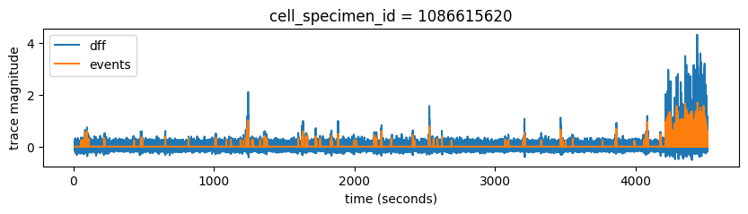
We can see that as expected, events trace is much cleaner than dff and it generally follows big Ca transients really well. We can also see that this cell was not very active during our experiment. Each experiment has a 5 minute movie at the end, which often drives neural activity really well. We can see a notable increase in cell’s activity at the end of this experiment.
Stimulus presentations#
The stimulus_presentations table contains one entry for each stimulus that was presented during the session, along with important metadata including stimulus start_time and end_time, as well as image_name.
During training, the only type of stimulus shown is in the context of the change detection task. During ophys sessions, there are additional stimulus periods before and after change detection task performance. stimulus_block and stimulus_block_name indicate the type of stimulus mice were presented at a given point in a session.
During the change_detection_behavior blocks,
and whether the stimulus was an image change (is_change = True) or an image omission (omitted = True).
To select active change detection behavior, first we need to filter the table for stimulus_block_name = change_detection_behavior or stimulus_block = 1. Note that different sessions may have different number of stimulus blocks, thus change_detection_behavior may be assosiated with either 0 or 1 in stimulus_block column.
Get stimulus information for this experiment and assign it to a table called stimulus_table.
Note the stimulus_block_name column. What are the unique values of stimulus_block_name?
stimulus_table = ophys_experiment.stimulus_presentations.copy()
print(stimulus_table.stimulus_block_name.unique())
stimulus_table.head(10)
['initial_gray_screen_5min' 'change_detection_behavior'
 'post_behavior_gray_screen_5min' 'natural_movie_one']
| stimulus_block | stimulus_block_name | image_index | image_name | movie_frame_index | duration | start_time | end_time | start_frame | end_frame | is_change | is_image_novel | omitted | movie_repeat | flashes_since_change | trials_id | active | is_sham_change | stimulus_name | |
|---|---|---|---|---|---|---|---|---|---|---|---|---|---|---|---|---|---|---|---|
| stimulus_presentations_id | |||||||||||||||||||
| 0 | 0 | initial_gray_screen_5min | -99 | NaN | -99 | 308.772448 | 0.000000 | 308.772448 | 0 | 17985 | False | <NA> | <NA> | -99 | 0 | -99 | False | False | spontaneous |
| 1 | 1 | change_detection_behavior | 0 | im000 | -99 | 0.250210 | 308.772448 | 309.022658 | 17985 | 18000 | False | True | False | -99 | 1 | 0 | True | False | Natural_Images_Lum_Matched_set_ophys_6_2017 |
| 2 | 1 | change_detection_behavior | 0 | im000 | -99 | 0.250180 | 309.523058 | 309.773238 | 18030 | 18045 | False | True | False | -99 | 2 | 0 | True | False | Natural_Images_Lum_Matched_set_ophys_6_2017 |
| 3 | 1 | change_detection_behavior | 0 | im000 | -99 | 0.250160 | 310.273688 | 310.523848 | 18075 | 18090 | False | True | False | -99 | 3 | 1 | True | False | Natural_Images_Lum_Matched_set_ophys_6_2017 |
| 4 | 1 | change_detection_behavior | 0 | im000 | -99 | 0.250220 | 311.024258 | 311.274478 | 18120 | 18135 | False | True | False | -99 | 4 | 1 | True | False | Natural_Images_Lum_Matched_set_ophys_6_2017 |
| 5 | 1 | change_detection_behavior | 0 | im000 | -99 | 0.250210 | 311.774888 | 312.025098 | 18165 | 18180 | False | True | False | -99 | 5 | 1 | True | False | Natural_Images_Lum_Matched_set_ophys_6_2017 |
| 6 | 1 | change_detection_behavior | 0 | im000 | -99 | 0.250150 | 312.525538 | 312.775688 | 18210 | 18225 | False | True | False | -99 | 6 | 1 | True | False | Natural_Images_Lum_Matched_set_ophys_6_2017 |
| 7 | 1 | change_detection_behavior | 0 | im000 | -99 | 0.250210 | 313.276118 | 313.526328 | 18255 | 18270 | False | True | False | -99 | 7 | 1 | True | False | Natural_Images_Lum_Matched_set_ophys_6_2017 |
| 8 | 1 | change_detection_behavior | 6 | im031 | -99 | 0.250220 | 314.026728 | 314.276948 | 18300 | 18315 | True | True | False | -99 | 0 | 1 | True | False | Natural_Images_Lum_Matched_set_ophys_6_2017 |
| 9 | 1 | change_detection_behavior | 6 | im031 | -99 | 0.250190 | 314.777358 | 315.027548 | 18345 | 18360 | False | True | False | -99 | 1 | 1 | True | False | Natural_Images_Lum_Matched_set_ophys_6_2017 |
Select the change_detection_behavior block, which is the portion of the session where mice perform the change detection task.
stimulus_table = stimulus_table[stimulus_table.stimulus_block_name=='change_detection_behavior']
stimulus_table.head(10)
| stimulus_block | stimulus_block_name | image_index | image_name | movie_frame_index | duration | start_time | end_time | start_frame | end_frame | is_change | is_image_novel | omitted | movie_repeat | flashes_since_change | trials_id | active | is_sham_change | stimulus_name | |
|---|---|---|---|---|---|---|---|---|---|---|---|---|---|---|---|---|---|---|---|
| stimulus_presentations_id | |||||||||||||||||||
| 1 | 1 | change_detection_behavior | 0 | im000 | -99 | 0.25021 | 308.772448 | 309.022658 | 17985 | 18000 | False | True | False | -99 | 1 | 0 | True | False | Natural_Images_Lum_Matched_set_ophys_6_2017 |
| 2 | 1 | change_detection_behavior | 0 | im000 | -99 | 0.25018 | 309.523058 | 309.773238 | 18030 | 18045 | False | True | False | -99 | 2 | 0 | True | False | Natural_Images_Lum_Matched_set_ophys_6_2017 |
| 3 | 1 | change_detection_behavior | 0 | im000 | -99 | 0.25016 | 310.273688 | 310.523848 | 18075 | 18090 | False | True | False | -99 | 3 | 1 | True | False | Natural_Images_Lum_Matched_set_ophys_6_2017 |
| 4 | 1 | change_detection_behavior | 0 | im000 | -99 | 0.25022 | 311.024258 | 311.274478 | 18120 | 18135 | False | True | False | -99 | 4 | 1 | True | False | Natural_Images_Lum_Matched_set_ophys_6_2017 |
| 5 | 1 | change_detection_behavior | 0 | im000 | -99 | 0.25021 | 311.774888 | 312.025098 | 18165 | 18180 | False | True | False | -99 | 5 | 1 | True | False | Natural_Images_Lum_Matched_set_ophys_6_2017 |
| 6 | 1 | change_detection_behavior | 0 | im000 | -99 | 0.25015 | 312.525538 | 312.775688 | 18210 | 18225 | False | True | False | -99 | 6 | 1 | True | False | Natural_Images_Lum_Matched_set_ophys_6_2017 |
| 7 | 1 | change_detection_behavior | 0 | im000 | -99 | 0.25021 | 313.276118 | 313.526328 | 18255 | 18270 | False | True | False | -99 | 7 | 1 | True | False | Natural_Images_Lum_Matched_set_ophys_6_2017 |
| 8 | 1 | change_detection_behavior | 6 | im031 | -99 | 0.25022 | 314.026728 | 314.276948 | 18300 | 18315 | True | True | False | -99 | 0 | 1 | True | False | Natural_Images_Lum_Matched_set_ophys_6_2017 |
| 9 | 1 | change_detection_behavior | 6 | im031 | -99 | 0.25019 | 314.777358 | 315.027548 | 18345 | 18360 | False | True | False | -99 | 1 | 1 | True | False | Natural_Images_Lum_Matched_set_ophys_6_2017 |
| 10 | 1 | change_detection_behavior | 6 | im031 | -99 | 0.25020 | 315.527958 | 315.778158 | 18390 | 18405 | False | True | False | -99 | 2 | 1 | True | False | Natural_Images_Lum_Matched_set_ophys_6_2017 |
How many unique images were shown?
print(stimulus_table.image_name.unique())
['im000' 'im031' 'omitted' 'im054' 'im073' 'im106' 'im075' 'im045' 'im035']
How many stimuli were omitted?
print('This experiment had {} stimuli.'.format(len(stimulus_table)))
print('Out of all stimuli presented, {} were omitted.'.format(len(stimulus_table[stimulus_table['image_name']=='omitted'])))
This experiment had 4797 stimuli.
Out of all stimuli presented, 160 were omitted.
dataframe columns:
- stimulus_presentations_id [index]
(int) identifier for a stimulus presentation (presentation of an image)
- stimulus_block_name
(str) name of each stimulus block indicating whether it is a gray screen (spontaneous activity period), change detection behavior task performance, or display of a natural movie
- stimulus_block
(int) index corresponding to
stimulus_block_name- image_name
(str) Indicates which natural scene image stimulus was shown for this stimulus presentation. Value will be NaN for all stimulus blocks other than
change_detection_behavior- image_index
(int) image index (0-7) for a given session, corresponding to each image name
- movie_frame_index
(int) index corresponding to the frame in the natural movie that was displayed at the end of some sessions; value will be -99 for all stimulus blocks other than
natural_movie_one- duration
(float) the duration, in seconds, of each stimulus presentation or spontaneous activity period; equivalent to
stop_time-start_time- start_time
(float) image presentation start time in seconds
- end_time
(float) image presentation end time in seconds
- start_frame
(int) image presentation start frame
- end_frame
(float) image presentation end frame
- is_change
(bool) whether the stimulus identity changed for this stimulus presentation
- is_image_novel
(bool) whether the stimulus presentation is an image from the novel (untrained) image set (does not indicate the very first presentation of a given image)
- omitted
(bool) True if no image was shown for this stimulus presentation
- movie_repeat
(int) index indicating the order of repeatitions of the 30 second movie clip in the natural_movie_one stimulus block (0-9); value will be -99 for other stimulus blocks
- flashes_since_change
float indicates how many flashes of the same image have occurred since the last stimulus change; values will be NaN for stimulus blocks other than
change_detection_behavior- trials_id
(int) Id to match to the table Index of the
trialstable- active
(bool) whether the stimulus presentation is part of an active behavior block (i.e mouse performing change detection task, not passive replay)
- stimulus_name
(str) name of the stimulus set used for the current stimulus block
- is_sham_change
(bool) whether the current stimulus presentation could have been a change based on the change time distribution; can be considered as “no-go” trials and used to quantify false alarms
Let’s explore the stimulus_presentations for the natural_movie_one stimulus block. Select the natural_movie_one block and inspect the unique values of image_name, movie_repeat, and movie_frame_index.
movie_stimulus_table = stimulus_table[stimulus_table.stimulus_block_name=='natural_movie_one']

print('Values of `image_name` are:', movie_stimulus_table.image_name.unique())
print('Values of `movie_repeat` are:', movie_stimulus_table.movie_repeat.unique())
print('Values of `movie_frame_index` are:', movie_stimulus_table.movie_frame_index.unique())
Values of `image_name` are: []
Values of `movie_repeat` are: []
Values of `movie_frame_index` are: []
To visualize the frames of natural_movie_one you can use the get_natural_movie_template method of the VisualBehaviorOphysProjectCache. This function can take a long time to run, since the movie has many frames. Here we will show how to use the function, but comment it out, to save time.
# movie_template = cache.get_natural_movie_template()
You can also download the full raw movie as an ndarray using the get_raw_natural_movie method.
Stimulus templates#
The stimulus_templates attribute is a dataframe containing one row per stimulus shown during the change detection task. The index is the image_name. The columns contain numpy arrays of the stimuli that were shown during the session.
The unwarped images represent the stimuli as they were seen by the mouse after correcting for distance from the mouse eye to the screen. The warped images show the exact image that was displayed on the stimulus monitor after spherical warping was applied to account for distance from the mouse’s eye.
ophys_experiment.stimulus_templates
| unwarped | warped | |
|---|---|---|
| image_name | ||
| im000 | [[nan, nan, nan, nan, nan, nan, nan, nan, nan,... | [[122, 122, 123, 125, 126, 127, 128, 129, 130,... |
| im106 | [[nan, nan, nan, nan, nan, nan, nan, nan, nan,... | [[108, 109, 106, 103, 102, 104, 107, 112, 117,... |
| im075 | [[nan, nan, nan, nan, nan, nan, nan, nan, nan,... | [[120, 121, 121, 121, 122, 123, 123, 122, 121,... |
| im073 | [[nan, nan, nan, nan, nan, nan, nan, nan, nan,... | [[120, 120, 118, 116, 116, 119, 121, 120, 117,... |
| im045 | [[nan, nan, nan, nan, nan, nan, nan, nan, nan,... | [[10, 13, 6, 0, 0, 8, 15, 13, 6, 2, 4, 9, 12, ... |
| im054 | [[nan, nan, nan, nan, nan, nan, nan, nan, nan,... | [[124, 125, 127, 130, 133, 134, 136, 138, 140,... |
| im031 | [[nan, nan, nan, nan, nan, nan, nan, nan, nan,... | [[233, 234, 244, 253, 253, 244, 237, 239, 246,... |
| im035 | [[nan, nan, nan, nan, nan, nan, nan, nan, nan,... | [[178, 181, 189, 198, 200, 198, 196, 199, 205,... |
stimulus_templates = ophys_experiment.stimulus_templates.copy()
stimuli = stimulus_templates.index.values
plt.imshow(stimulus_templates.loc[stimuli[0]]['unwarped'], cmap='gray')
<matplotlib.image.AxesImage at 0x7fb4781aec80>
Stimulus timestamps#
All behavioral measurements (running_speed, licks, & rewards) are made at the frequency of visual stimulus display (60Hz) and share frame times with the stimulus_presentations. You can use the frame index from any of the other behavior tables to determine the corresponding timestamp.
ophys_experiment.stimulus_timestamps
array([   8.74134,    8.75801,    8.77469, ..., 4510.21911, 4510.23578,
       4510.25249])
Lick times#
The licks attribute is a dataframe with one entry for every detected lick onset time, assigned the time of the corresponding visual stimulus frame.
ophys_experiment.licks.sample(5)
| timestamps | frame | |
|---|---|---|
| 2322 | 1762.59091 | 105145 |
| 2457 | 1889.39452 | 112747 |
| 2765 | 2382.73098 | 142323 |
| 1952 | 1543.94562 | 92037 |
| 2216 | 1722.14121 | 102720 |
Rewards#
The rewards attribute is a dataframe containing one entry for every reward that was delivered, assigned the time of the corresponding visual stimulus frame. auto_rewarded is True if the reward was delivered without requiring a preceding lick. The first 5 change trials of each session are auto_rewarded = True.
ophys_experiment.rewards.sample(5)
| volume | timestamps | auto_rewarded | |
|---|---|---|---|
| 16 | 0.007 | 1013.37880 | False |
| 33 | 0.007 | 1487.86647 | False |
| 57 | 0.007 | 1902.20501 | False |
| 65 | 0.007 | 2045.57213 | False |
| 39 | 0.007 | 1612.98536 | False |
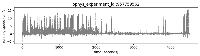
Running speed#
Mice are free to run on a circular disc during task performance. The running_speed table contains one entry for each read of the analog input line monitoring the encoder voltage, measured at 60 Hz. running_speed shares timestamps with the stimulus, provided in the stimulus_timestamps attribute.
ophys_experiment.running_speed.head()
| timestamps | speed | |
|---|---|---|
| 0 | 8.74134 | -0.006992 |
| 1 | 8.75801 | 0.389996 |
| 2 | 8.77469 | 0.754625 |
| 3 | 8.79138 | 1.057696 |
| 4 | 8.80804 | 1.277703 |
Plot the mouse’s running_speed for this experiment.
fig, ax = plt.subplots(1,1, figsize = (10,2))
ax.plot(ophys_experiment.stimulus_timestamps, ophys_experiment.running_speed['speed'], color='gray', linestyle='--')
ax.set_xlabel('time (seconds)')
ax.set_ylabel('running speed (cm/s)')
ax.set_title('ophys_experiment_id :'+str(ophys_experiment_id))
Text(0.5, 1.0, 'ophys_experiment_id :957759562')
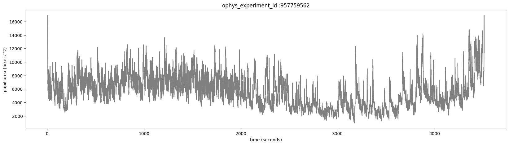
Eye tracking#
The eye_tracking table containing ellipse fit parameters for the eye, pupil and corneal reflection (cr). Fits are derived from tracking points from a DeepLabCut model applied to video frames of the mouse’s right eye (collected at 60hz). The pupil_area is the total area, in pixels, of the ellipse fit.
The corneal reflection (cr) fit can be used to estimate the axis of the camera. Taking the difference between the corneal reflection position and the pupil position can therefore disambiguate translations of the entire eye (in which case both the cr and pupil will shift together) from rotations of the eye (in which case the pupil position will move relative to the corneal reflection).
Examine the eye_tracking table
ophys_experiment.eye_tracking.head()
| timestamps | cr_area | eye_area | pupil_area | likely_blink | pupil_area_raw | cr_area_raw | eye_area_raw | cr_center_x | cr_center_y | ... | eye_center_x | eye_center_y | eye_width | eye_height | eye_phi | pupil_center_x | pupil_center_y | pupil_width | pupil_height | pupil_phi | |
|---|---|---|---|---|---|---|---|---|---|---|---|---|---|---|---|---|---|---|---|---|---|
| frame | |||||||||||||||||||||
| 0 | 0.17278 | NaN | NaN | NaN | True | 23212.800552 | 98.711757 | 64631.264284 | 348.546244 | 279.151509 | ... | 360.406224 | 259.823698 | NaN | NaN | NaN | 351.118771 | 268.126167 | NaN | NaN | NaN |
| 1 | 0.20753 | NaN | NaN | NaN | True | 23268.865872 | 98.428380 | 64589.149589 | 348.537688 | 279.138556 | ... | 360.304902 | 260.023828 | NaN | NaN | NaN | 351.379090 | 268.190725 | NaN | NaN | NaN |
| 2 | 0.20986 | NaN | NaN | NaN | True | 23322.880481 | 108.124556 | 64667.735921 | 348.776906 | 278.763494 | ... | 360.768207 | 258.962922 | NaN | NaN | NaN | 350.680601 | 268.043758 | NaN | NaN | NaN |
| 3 | 0.24332 | NaN | NaN | NaN | True | 23465.541426 | 109.606476 | 64536.922664 | 348.503846 | 278.154595 | ... | 361.383089 | 258.391708 | NaN | NaN | NaN | 351.469294 | 268.284240 | NaN | NaN | NaN |
| 4 | 0.28209 | NaN | NaN | NaN | True | 23404.595038 | 106.169282 | 64285.566594 | 348.358439 | 277.939624 | ... | 360.861868 | 257.989534 | NaN | NaN | NaN | 351.004937 | 268.315566 | NaN | NaN | NaN |
5 rows × 23 columns
dataframe columns:
- frame (index)
(int) frame of eye tracking video.
- timestamps
(float) experiment timestamp for frame in seconds
- cr_area
(float) area of corneal reflection ellipse in pixels squared
- eye_area
(float) area of eye ellipse in pixels squared
- pupil_area
(float) area of pupil ellipse in pixels squared
- likely_blink
(bool) True if frame has outlier ellipse fits, which is often caused by blinking / squinting of the eye.
- eye_area_raw
(float) pupil area with no outliers/likely blinks removed.
- eye_center_x
(float) center of eye ellipse on x axis in pixels
- eye_center_y
(float) center of eye ellipse on y axis in pixels
- eye_height
(float) eye height (minor axis of the eye ellipse) in pixels
- eye_width
(float) eye width (major axis of the eye ellipse) in pixels
- eye_phi
(float) eye rotation angle in radians
- pupil_area_raw
(float) pupil area with no outliers/likely blinks removed.
- pupil_center_x
(float) center of pupil ellipse on x axis in pixels
- pupil_center_y
(float) center of pupil ellipse on y axis in pixels
- pupil_height
(float) pupil height (minor axis of the pupil ellipse) in pixels
- pupil_width
(float) pupil width (major axis of the pupil ellipse) in pixels
- pupil_phi
(float) pupil rotation angle in radians
- cr_area_raw
(float) corneal reflection area with no outliers/likely blinks removed.
- cr_center_x
(float) center of corneal reflection on x axis in pixels
- cr_center_y
(float) center of corneal reflection on y axis in pixels
- cr_height
(float) corneal reflection height (minor axis of the CR ellipse) in pixels
- cr_width
(float) corneal reflection width (major axis of the CR ellipse) in pixels
- cr_phi
(float) corneal reflection rotation angle in radians
Plot the pupil_area for this experiment.
fig, ax = plt.subplots(1,1, figsize = (20,5))
ax.plot(ophys_experiment.eye_tracking.timestamps, ophys_experiment.eye_tracking.pupil_area, color='gray')
ax.set_xlabel('time (seconds)')
ax.set_ylabel('pupil area (pixels^2)')
ax.set_title('ophys_experiment_id :'+str(ophys_experiment_id))
Text(0.5, 1.0, 'ophys_experiment_id :957759562')
Task parameters#
The task_parameters attribute contains information about the structure of the behavior task for that specific session.
ophys_experiment.task_parameters
{'auto_reward_volume': 0.005,
 'blank_duration_sec': [0.5, 0.5],
 'image_set': 'images_B',
 'n_stimulus_frames': 69575,
 'omitted_flash_fraction': 0.05,
 'response_window_sec': [0.15, 0.75],
 'reward_volume': 0.007,
 'session_type': 'OPHYS_4_images_B',
 'stimulus': 'images',
 'stimulus_distribution': 'geometric',
 'stimulus_duration_sec': 0.25,
 'stimulus_name': 'Natural_Images_Lum_Matched_set_ophys_6_2017',
 'task': 'change detection'}
Here we can see that the stimulus_duration_sec is 0.25 seconds and the blank_duration_sec is 0.5 seconds. This determines the inter-stimulus interval.
dataframe columns:
- auto_reward_volume
(float) Volume of auto rewards in ml.
- blank_duration_sec
(list of floats) Duration in seconds of inter stimulus interval. Inter-stimulus interval chosen as a uniform random value between the range defined by the two values. Values are ignored if
stimulus_duration_secis null.- response_window_sec
(list of floats) Range of period following an image change, in seconds, where mouse response influences trial outcome. First value represents response window start. Second value represents response window end. Values represent time before display lag is accounted for and applied.
- n_stimulus_frames
(int) Total number of visual stimulus frames presented during a behavior session.
- task
(string) Type of behavioral task (‘change_detection’ for this dataset)
- session_type
(string) Visual stimulus type run during behavior session.
- omitted_flash_fraction
(float) Probability that a stimulus image presentations is omitted. Change stimuli, and the stimulus immediately preceding the change, are never omitted.
- stimulus_distribution
(string) Distribution for drawing change times. Either ‘exponential’ or ‘geometric’.
- stimulus_duration_sec
(float) Duration in seconds of each stimulus image presentation
- reward_volume
(float) Volume of earned water reward in ml.
- stimulus
(string) Stimulus type (‘gratings’ or ‘images’).
Trials#
While the stimulus_presentations table has one entry for each individual stimulus that was presented, the trials table contains one entry for each behavioral trial, which consists of a series of stimulus presentations and is defined by the change_time.
On a given trial, a change_time is selected from a geometric distribution between 4 and 12 flashes after the time of the last change or the last lick.
On go trials, the image identity will change at the selected change_time. If the mouse licks within the response window (see response_window_sec entry of the `task_parameters attribute), that is considered a hit and a reward will be delivered. If the mouse fails to lick after the change, the trial is considered a miss.
On catch trials, a change_time is drawn, but the image identity does not change. If the mouse licks within the reward window, this is a false alarm and no reward is delivered. Correctly withholding a lick is called a correct reject.
This definition of a catch trial is a conservative one, and only considers the non-change stimulus presentations that are drawn from the same distribution as the change times. A less restrictive definition could consider every non-change stimulus presentation as a catch trial, and the false alarm rate can be computed this way as well.
If the mouse licks prior to the scheduled change_time, the trial is aborted and starts over again, using the same change_time for up to 5 trials in a row. This is to discourage mice from licking frequently, as they have to wait until the change time to get a reward.
# look at 5 random trials
ophys_experiment.trials.sample(5)
| start_time | stop_time | initial_image_name | change_image_name | is_change | change_time | go | catch | lick_times | response_time | ... | reward_time | reward_volume | hit | false_alarm | miss | correct_reject | aborted | auto_rewarded | change_frame | trial_length | |
|---|---|---|---|---|---|---|---|---|---|---|---|---|---|---|---|---|---|---|---|---|---|
| trials_id | |||||||||||||||||||||
| 586 | 3434.02329 | 3443.54770 | im000 | im045 | True | 3439.313528 | True | False | [] | NaN | ... | NaN | 0.0 | False | False | True | False | False | False | 205664 | 9.52441 |
| 386 | 2021.81940 | 2032.09447 | im106 | im106 | False | 2027.860278 | False | True | [] | NaN | ... | NaN | 0.0 | False | False | False | True | False | False | 121046 | 10.27507 |
| 428 | 2329.65433 | 2336.92687 | im045 | im031 | True | 2332.692708 | True | False | [] | NaN | ... | NaN | 0.0 | False | False | True | False | False | False | 139321 | 7.27254 |
| 601 | 3559.37566 | 3568.90012 | im075 | im000 | True | 3564.665968 | True | False | [] | NaN | ... | NaN | 0.0 | False | False | True | False | False | False | 213179 | 9.52446 |
| 246 | 1241.86549 | 1245.88544 | im045 | im045 | False | NaN | False | False | [1245.40168, 1245.56851] | NaN | ... | NaN | 0.0 | False | False | False | False | True | False | -99 | 4.01995 |
5 rows × 21 columns
dataframe columns:
- start_time
(float) Experiment time when this trial began in seconds.
- stop_time
(float) Experiment time when this trial ended.
- lick_times
(float array) A list indicating when the behavioral control software recognized a lick. Note that this is not identical to the lick times from the licks dataframe, which record when the licks were registered by the lick sensor. The licks dataframe should generally be used for analysis of the licking behavior rather than these times.
- reward_time
(float) Indicates when the reward command was triggered for hit trials. NaN for other trial types.
- reward_volume
(float) Indicates the volume of water dispensed as reward for this trial.
- is_change
(bool) Indicates whether an image change occurred for this trial.
- change_time
(float) The time when the change in image identity occurs. This change time is used to determine the response window during which a lick will trigger a reward.
- change_frame
(int) Indicates the stimulus frame index when the change (on go trials) or sham change (on catch trials) occurred. This column can be used to link the trials table with the stimulus presentations table, as shown below.
- go
(bool) Indicates whether this trial was a ‘go’ trial. To qualify as a go trial, an image change must occur and the trial cannot be autorewarded.
- catch
(bool) Indicates whether this trial was a ‘catch’ trial. To qualify as a catch trial, a ‘sham’ change must occur during which the image identity does not change. These sham changes are drawn to match the timing distribution of real changes and can be used to calculate the false alarm rate.
- hit
(bool) Indicates whether this trial was a ‘hit’ trial. To qualify as a hit, the trial must be a go trial during which the stimulus changed and the mouse licked within the reward window (150-750 ms after the change time).
- false_alarm
(bool) Indicates whether this trial was a ‘false alarm’ trial. To qualify as a false alarm, the trial must be a catch trial during which a sham change occurred and the mouse licked during the reward window.
- miss
(bool) To qualify as a miss trial, the trial must be a go trial during which the stimulus changed but the mouse did not lick within the response window.
- correct_reject
(bool) To qualify as a correct reject trial, the trial must be a catch trial during which a sham change occurred and the mouse withheld licking.
- aborted
(bool) A trial is aborted when the mouse licks before the scheduled change or sham change.
- auto_rewarded
(bool) During autorewarded trials, the reward is automatically triggered after the change regardless of whether the mouse licked within the response window. These always come at the beginning of the session to help engage the mouse in behavior.
- initial_image_name
(float) Indicates which image was shown before the change (or sham change) for this trial
- change_image_name
(string) Indicates which image was scheduled to be the change image for this trial. Note that if the trial is aborted, a new trial will begin before this change occurs.
- trial_length
(float) Duration of the trial in seconds.
- response_time
(float) Indicates the time when the first lick was registered by the task control software for trials that were not aborted (go or catch). NaN for aborted trials. For a more accurate measure of response time, the licks dataframe should be used.
Performance metrics#
One useful method of the ophys_experiment object is the get_performance_metrics method, which returns some summary metrics on the session.
# get behavior performance metrics for one session
ophys_experiment.get_performance_metrics()
{'trial_count': 640,
 'go_trial_count': 252,
 'catch_trial_count': 35,
 'hit_trial_count': 70,
 'miss_trial_count': 182,
 'false_alarm_trial_count': 2,
 'correct_reject_trial_count': 33,
 'auto_reward_count': 5,
 'earned_reward_count': 70,
 'total_reward_count': 75,
 'total_reward_volume': 0.515,
 'maximum_reward_rate': 4.3130202342807245,
 'engaged_trial_count': 212,
 'mean_hit_rate': 0.4252895970233363,
 'mean_hit_rate_uncorrected': 0.4256732205557432,
 'mean_hit_rate_engaged': 0.872856714153381,
 'mean_false_alarm_rate': 0.11763102364147658,
 'mean_false_alarm_rate_uncorrected': 0.07070533028721182,
 'mean_false_alarm_rate_engaged': 0.1913937670516618,
 'mean_dprime': 0.823586586603706,
 'mean_dprime_engaged': 2.0336866686070554,
 'max_dprime': 2.5554209406856407,
 'max_dprime_engaged': 2.5554209406856407}
You can also access performing metrics computed on a rolling basis across trials using the get_rolling_performance_df method. The rolling performance metrics share timestamps with the change_times of the trials table.
ophys_experiment.get_rolling_performance_df()
| reward_rate | hit_rate_raw | hit_rate | false_alarm_rate_raw | false_alarm_rate | rolling_dprime | |
|---|---|---|---|---|---|---|
| trials_id | ||||||
| 0 | NaN | NaN | NaN | NaN | NaN | NaN |
| 1 | NaN | NaN | NaN | NaN | NaN | NaN |
| 2 | NaN | NaN | NaN | NaN | NaN | NaN |
| 3 | NaN | NaN | NaN | NaN | NaN | NaN |
| 4 | NaN | NaN | NaN | NaN | NaN | NaN |
| ... | ... | ... | ... | ... | ... | ... |
| 635 | 0.0 | 0.0 | 0.005747 | 0.0 | 0.038462 | -0.557523 |
| 636 | 0.0 | 0.0 | 0.005682 | 0.0 | 0.041667 | -0.594683 |
| 637 | 0.0 | 0.0 | 0.005682 | 0.0 | 0.041667 | -0.594683 |
| 638 | 0.0 | 0.0 | 0.005682 | 0.0 | 0.041667 | -0.594683 |
| 639 | 0.0 | 0.0 | 0.005682 | 0.0 | 0.041667 | -0.594683 |
640 rows × 6 columns
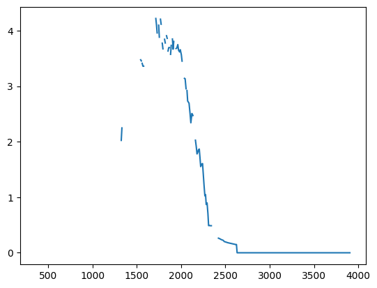
Plot the reward rate over time during the session.
performance_df = ophys_experiment.get_rolling_performance_df()
plt.plot(ophys_experiment.trials.change_time.values, performance_df.reward_rate.values)
[<matplotlib.lines.Line2D at 0x7fb475e19e70>]
Plot example cell activity with stimuli and behavior#
We can select a cell from the experiment and plot it’s dff_traces and events traces along with other behavioral and stimulus data, including running_speed, pupil_area, as well as stimulus timing using the stimulus_presentations table.
Below we will put together plotting functions that utilize data from the ophys_experiment object to plot ophys traces and behavioral data from the experiment.
First, get stimulus information.
# create a list of all unique stimuli presented in this experiment
unique_stimuli = [stimulus for stimulus in stimulus_table['image_name'].unique()]

# create a colormap with each unique image having its own color
colormap = {image_name: sns.color_palette()[image_number] for image_number, image_name in enumerate(np.sort(unique_stimuli))}
colormap['omitted'] = (1,1,1) # set omitted stimulus to white color

# add the colors for each image to the stimulus presentations table in the dataset
stimulus_presentations = stimulus_table.copy()
stimulus_presentations['color'] = stimulus_presentations['image_name'].map(lambda image_name: colormap[image_name])
Here are some plotting functions for convenience.
# function to plot dff traces
def plot_dff_trace(ax, cell_specimen_id, initial_time, final_time):
    '''
        ax: axis on which to plot
        cell_specimen_id: id of the cell to plot
        initial_time: initial time to plot from
        final_time: final time to plot to
    '''
    #create a dataframe using dff trace from one selected cell
    data = {'dff': ophys_experiment.dff_traces.loc[cell_specimen_id]['dff'],
        'timestamps': ophys_experiment.ophys_timestamps}
    df = pd.DataFrame(data)
    dff_trace_sample = df[(df.timestamps >= initial_time) & (df.timestamps <= final_time)]
    ax.plot(dff_trace_sample['timestamps'], dff_trace_sample['dff']/dff_trace_sample['dff'].max())

# function to plot events traces
def plot_events_trace(ax, cell_specimen_id, initial_time, final_time):
    # create a dataframe using events trace from one selected cell
    data = {'events': ophys_experiment.events.loc[cell_specimen_id].events,
        'timestamps': ophys_experiment.ophys_timestamps}
    df = pd.DataFrame(data)
    events_trace_sample = df[(df.timestamps >= initial_time) & (df.timestamps <= final_time)]
    ax.plot(events_trace_sample['timestamps'], events_trace_sample['events']/events_trace_sample['events'].max())

# function to plot running speed
def plot_running(ax, initial_time, final_time):
    running_sample = ophys_experiment.running_speed.copy()
    running_sample = running_sample[(running_sample.timestamps >= initial_time) & (running_sample.timestamps <= final_time)]
    ax.plot(running_sample['timestamps'], running_sample['speed']/running_sample['speed'].max(),
            '--', color = 'gray', linewidth = 1)

# function to plot pupil diameter
def plot_pupil(ax, initial_time, final_time):
    pupil_sample = ophys_experiment.eye_tracking.copy()
    pupil_sample = pupil_sample[(pupil_sample.timestamps >= initial_time) &
                                (pupil_sample.timestamps <= final_time)]
    ax.plot(pupil_sample['timestamps'], pupil_sample['pupil_width']/pupil_sample['pupil_width'].max(),
            color = 'gray', linewidth = 1)

# function to plot licks
def plot_licks(ax, initial_time, final_time):
    licking_sample = ophys_experiment.licks.copy()
    licking_sample = licking_sample[(licking_sample.timestamps >= initial_time) &
                                    (licking_sample.timestamps <= final_time)]
    ax.plot(licking_sample['timestamps'], np.zeros_like(licking_sample['timestamps']),
            marker = 'o', markersize = 3, color = 'black', linestyle = 'none')

# function to plot rewards
def plot_rewards(ax, initial_time, final_time):
    rewards_sample = ophys_experiment.rewards.copy()
    rewards_sample = rewards_sample[(rewards_sample.timestamps >= initial_time) &
                                    (rewards_sample.timestamps <= final_time)]
    ax.plot(rewards_sample['timestamps'], np.zeros_like(rewards_sample['timestamps']),
            marker = 'd', color = 'blue', linestyle = 'none', markersize = 12, alpha = 0.5)

# function to plot stimuli
def plot_stimuli(ax, initial_time, final_time):
    stimulus_presentations_sample = stimulus_presentations.copy()
    stimulus_presentations_sample = stimulus_presentations_sample[(stimulus_presentations_sample.end_time >= initial_time) & (stimulus_presentations_sample.start_time <= final_time)]
    for idx, stimulus in stimulus_presentations_sample.iterrows():
        ax.axvspan(stimulus['start_time'], stimulus['end_time'], color=stimulus['color'], alpha=0.25)
Create the plot for one cell#
initial_time = 820 # start time in seconds
final_time = 860 # stop time in seconds

fig, ax = plt.subplots(2,1,figsize = (15,7))

plot_dff_trace(ax[0], cell_specimen_ids[3], initial_time, final_time)
plot_events_trace(ax[0], cell_specimen_ids[3], initial_time, final_time)
plot_stimuli(ax[0], initial_time, final_time)
ax[0].set_ylabel('normalized response magnitude')
ax[0].set_yticks([])
ax[0].legend(['dff trace', 'events trace'])

plot_running(ax[1], initial_time, final_time)
plot_pupil(ax[1], initial_time, final_time)
plot_licks(ax[1], initial_time, final_time)
plot_rewards(ax[1], initial_time, final_time)
plot_stimuli(ax[1], initial_time, final_time)

ax[1].set_yticks([])
ax[1].legend(['running speed', 'pupil','licks', 'rewards'])
<matplotlib.legend.Legend at 0x7fb4785e3580>
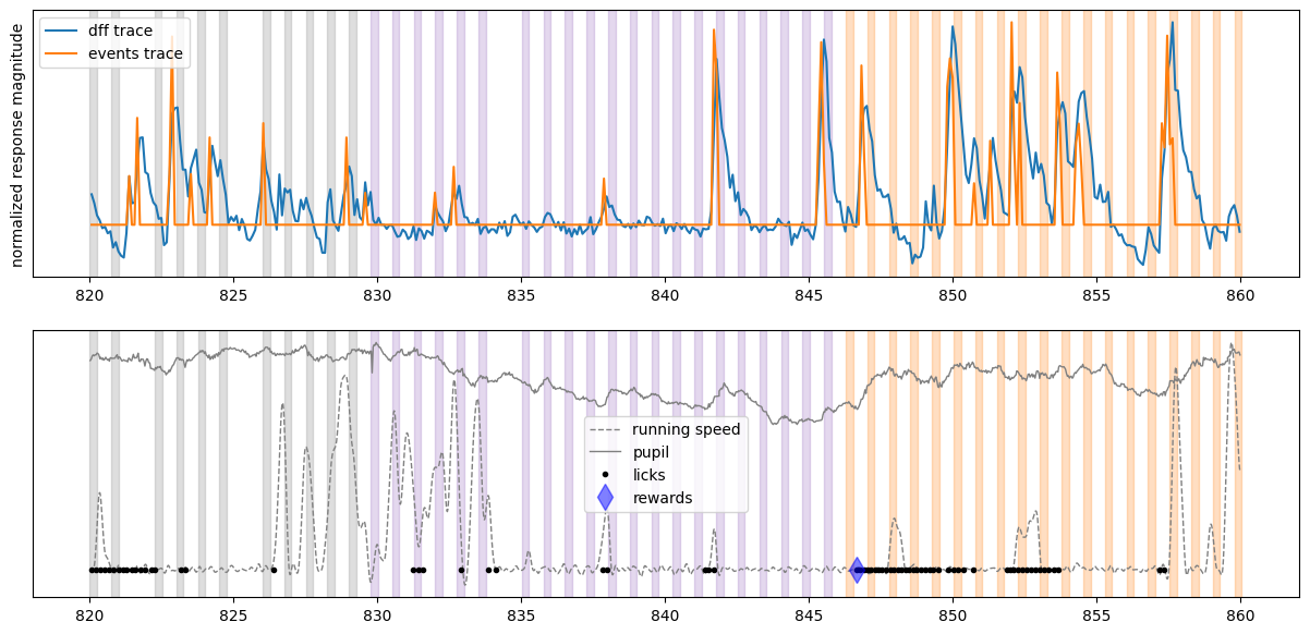
From looking at the activity of this neuron, we can see that it was very active during our experiment but its activity does not appear to be reliably locked to image presentations. It does seem to vaguely follow animal’s running speed, thus it might be modulated by running.
Create the same plot for a Vip cell from a different experiment#
We can get a different, Vip experiment from session_type = OPHYS_1 (equivalent to session_number = 1) and plot it to compare response traces. This gives us a similar plot from a different inhibitory neuron to compare their neural dynamics.
# Select a Vip experiment with familiar images (session_number = 1, 2, or 3)
selected_experiment_table = ophys_experiment_table[(ophys_experiment_table.cre_line=='Vip-IRES-Cre')&
                        (ophys_experiment_table.session_number==1)]

# load the experiment data from the cache
ophys_experiment = cache.get_behavior_ophys_experiment(selected_experiment_table.index.values[1])
# get the cell IDs
cell_specimen_ids = ophys_experiment.cell_specimen_table.index.values # a list of all cell ids
/opt/envs/allensdk/lib/python3.10/site-packages/hdmf/utils.py:668: UserWarning: Ignoring cached namespace 'core' version 2.6.0-alpha because version 2.7.0 is already loaded.
  return func(args[0], **pargs)
# create a list of all unique stimuli presented in this experiment
unique_stimuli = [stimulus for stimulus in stimulus_table['image_name'].unique()]

# create a colormap with each unique image having its own color
colormap = {image_name: sns.color_palette()[image_number] for image_number, image_name in enumerate(np.sort(unique_stimuli))}
colormap['omitted'] = (1,1,1)

# add the colors for each image to the stimulus presentations table in the dataset
stimulus_presentations = stimulus_table.copy()
stimulus_presentations['color'] = stimulus_presentations['image_name'].map(lambda image_name: colormap[image_name])
# we can plot the same information for a different cell in the dataset
initial_time = 580 # start time in seconds
final_time = 620 # stop time in seconds
fig, ax = plt.subplots(2,1,figsize = (15,7))

plot_dff_trace(ax[0], cell_specimen_ids[5], initial_time, final_time)
plot_events_trace(ax[0], cell_specimen_ids[5], initial_time, final_time)
plot_stimuli(ax[0], initial_time, final_time)
ax[0].set_ylabel('normalized response magnitude')
ax[0].set_yticks([])
ax[0].legend(['dff trace', 'events trace'])

plot_running(ax[1], initial_time, final_time)
plot_pupil(ax[1], initial_time, final_time)
plot_licks(ax[1], initial_time, final_time)
plot_rewards(ax[1], initial_time, final_time)
plot_stimuli(ax[1], initial_time, final_time)

ax[1].set_yticks([])
ax[1].legend(['running speed', 'pupil','licks', 'rewards'])
<matplotlib.legend.Legend at 0x7fb476215e40>
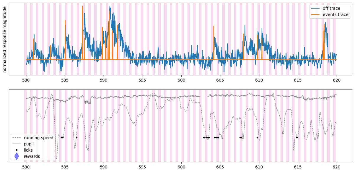
We can see that the dynamics of a Vip neuron are also not driven by the visual stimuli. Aligning neural activity to different behavioral or experimental events might reveal what this neuron is driven by.