This tutorial will cover the basics of analyzing data using regression using Python’s numpy and scikit-learn packages.

import numpy as np
import matplotlib.pyplot as plt
%matplotlib inline

Regression

Regression is a method of attempting to “fit” data to a function. The goal is, given a set of ordered pairs \((\vec{x_i}, y_i)\) where \(i \in \mathbb{Z}_0^+\), to construct a mapping \(f: X^n \rightarrow Y\) such that \(f(\vec{x}) \approx y\) for all \((\vec{x_i}, y_i)\). Obviously, there is an infinite number of such maps that could be constructed, so there is an inherent ambiguity in what the target function should be; moreover, the true, underlying relationship between the variables can never be exactly reconstructed from data due to measurement error and noise. The goal is not necessarily to recover the true relationship, then, but rather to construct an approximate model that can be used to accurately predict target values within some neighborhood of the data interval. Of course, if the model turns out to work across the entire domain, so much the better, but this will usually not be a realistic goal.

The simplest way of doing this is by using a linear regression. This attempts to approximate the underlying, true function as a linear combination of basis functions:

\(f(\vec{x_i}) = \sum_j w_j \phi_j(\vec{x_i})\)

The basis functions \(\phi_i\) may be any convenient choice and need not be orthogonal; one convenient (non-orthogonal) choice that is frequently used are polynomials, \(\phi_0(x_i) = 1\), \(\phi_1(x_i) = x_i\), \(\phi_2(x_i) = x_i^2\), …, \(\phi_n(x_i) = x_i^n\). Other convenient (orthogonal) bases that can be chosen include the Hermite polynomials or the Fourier basis (this is equivalent to performing a discrete Fourier transform). The basis functions are often referred to as “features”. Because the function is approximated as a weighted sum of these basis functions, their coefficients are then referred to as “weights”. One way to think of this is that the regression is like a Taylor expansion; but rather than knowing a true function and computing a series to approximate it, in regression, we assume that the underlying function can be series expanded and are recursively attempting to determine each term in the series.

{
    "tags": [
        "remove-input",
    ]
}

from scipy import special

def hermite_n(degree):
    return special.hermite(degree, monic=True)

x = np.linspace(-2, 2, 400)

plt.subplots(1, 2, figsize=(10,5))
ax1 = plt.subplot(1, 2, 1)

for i in range(5):
    y_i = hermite_n(i + 1)(x)
    plt.plot(x, y_i)

plt.xlabel('x')
plt.ylabel('y')
plt.title('First Five Hermite Polynomials')

def poly_n(input, degree):
    return input**degree

ax2 = plt.subplot(1, 2, 2)
ax2.set_ylim(-5, 5)
for i in range(5):
    y_i = poly_n(x, i+1)
    plt.plot(x, y_i)

plt.xlabel('x')
plt.ylabel('y')
plt.title('First Five Powers')

Text(0.5, 1.0, 'First Five Powers')

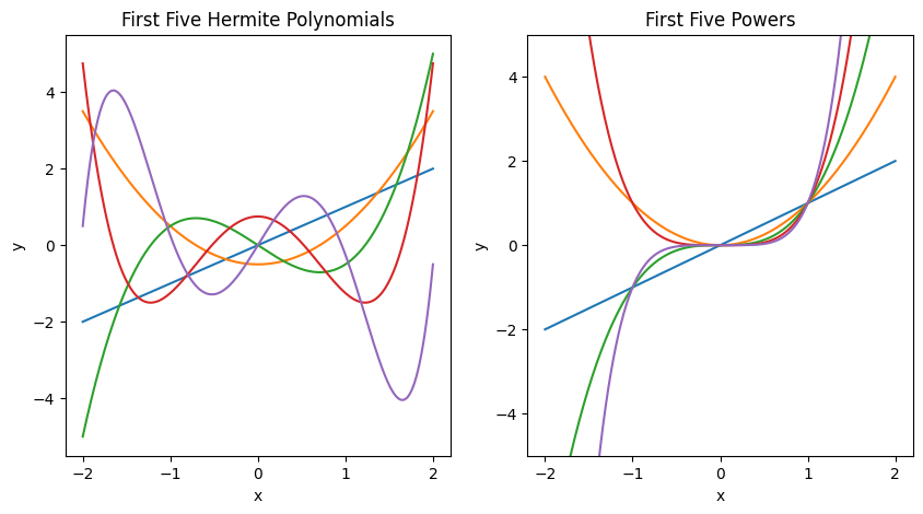
Fig. 1: On the left is shown the first five Hermite polynomials, which are one possible choice of an orthonormal basis for the space of square-integrable functions. On the right is shown the five first powers of x, which are another possible choice of basis for the same space, but are not orthonormal. Either of these could be chosen as bases for a regression, in addition to a myriad of other basis choices.

The simplest and most familiar type of linear regression is the fitting of one-dimensional data to a line, so that \(y = mx+b\) approximates the data (sometimes this is called finding a trendline).

The weights can be found using linear algebra or variationally, by defining an error function:

\(E = \frac{1}{2} |y_i - f(\vec{x_i})|^2 = \frac{1}{2}\sum_i|y_i - \sum_j w_j\phi_j(\vec{x_i})|^2\)

This function is the sum of squared errors. To understand how it captures the error, remember that we are choosing \(f(\vec{x_i})\) so that \(f(\vec{x_i}) \approx y_i\) but in general \(f(\vec{x_i}) \neq y_i\). The difference \(y_i - f(\vec{x_i})\) captures information about how much the approximation deviates at each point from the true value of the data. Since the differences could be negative or positive, we cannot sum them directly; terms where the approximation predicts a smaller value of y than the true value would cancel terms where the approximation predicts a larger value of y than the true value. We therefore square the deviations to make the error measure strictly non-negative, and sum the squares to get the total error, which is how well our approximation performs overall.

Finally, in order to do our regression, we choose how many terms we want in our regression (what the maximum value of j is), and then find the values of the weights \(w_j\) that minimize the error. An example will follow to make this clearer.

Example: Linear regression on a one-dimensional dataset

First, we will generate some fake data that we will then attempt to approximate. This is slightly unrealistic, since on a real dataset the best model to generate the data will not be known. The function that we shall use is:

\(F(x) = \text{2 Exp}(-5x)\)

This has been chosen since it is an exponential decay, which appears frequently in nature. We will also generate some data, which will have some random noise attached to it.

# Create the generating function

x0 = np.linspace(0,1.0, 100)

def f_true(xt): 
    return 2 * np.exp(-5 * xt)

# Plot it so we can see what it looks like
fig, ax = plt.subplots()
ax.plot(x0, f_true(x0))
ax.set_xlabel('x')
ax.set_ylabel('y')

# Generate some fake data
n = 200

x = np.sort(np.random.random(n))
y = f_true(x) + 0.2*np.random.normal(size=n)

# Plot the raw data
ax.plot(x, y, 'o', c='green')
plt.title('Generated Data and Generating Function')

Text(0.5, 1.0, 'Generated Data and Generating Function')

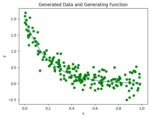
Above, we can see the fake data in green, and the true curve in blue. Now, we will attempt to fit the data using the above non-orthogonal choice of functions \(\phi_n = x^n\) (from here on, we suppress arguments of \(\phi_n\) for brevity). (There are some advantages to doing a regression using an orthogonal basis, but raw polynomials are often easier to interpret.) A quick definition of some verbiage: model generally refers to the choice of basis functions \(\phi_i\) we have selected, without any determination of what the weights are. Training generally refers to the computation of the coefficients \(w_i\) for a choice of model. A trained model is therefore the final function \(f(x_i) = \sum_j w_j \phi_j\) where \(w_j\) and \(\phi_j\) are both fully determined for all \(j\).

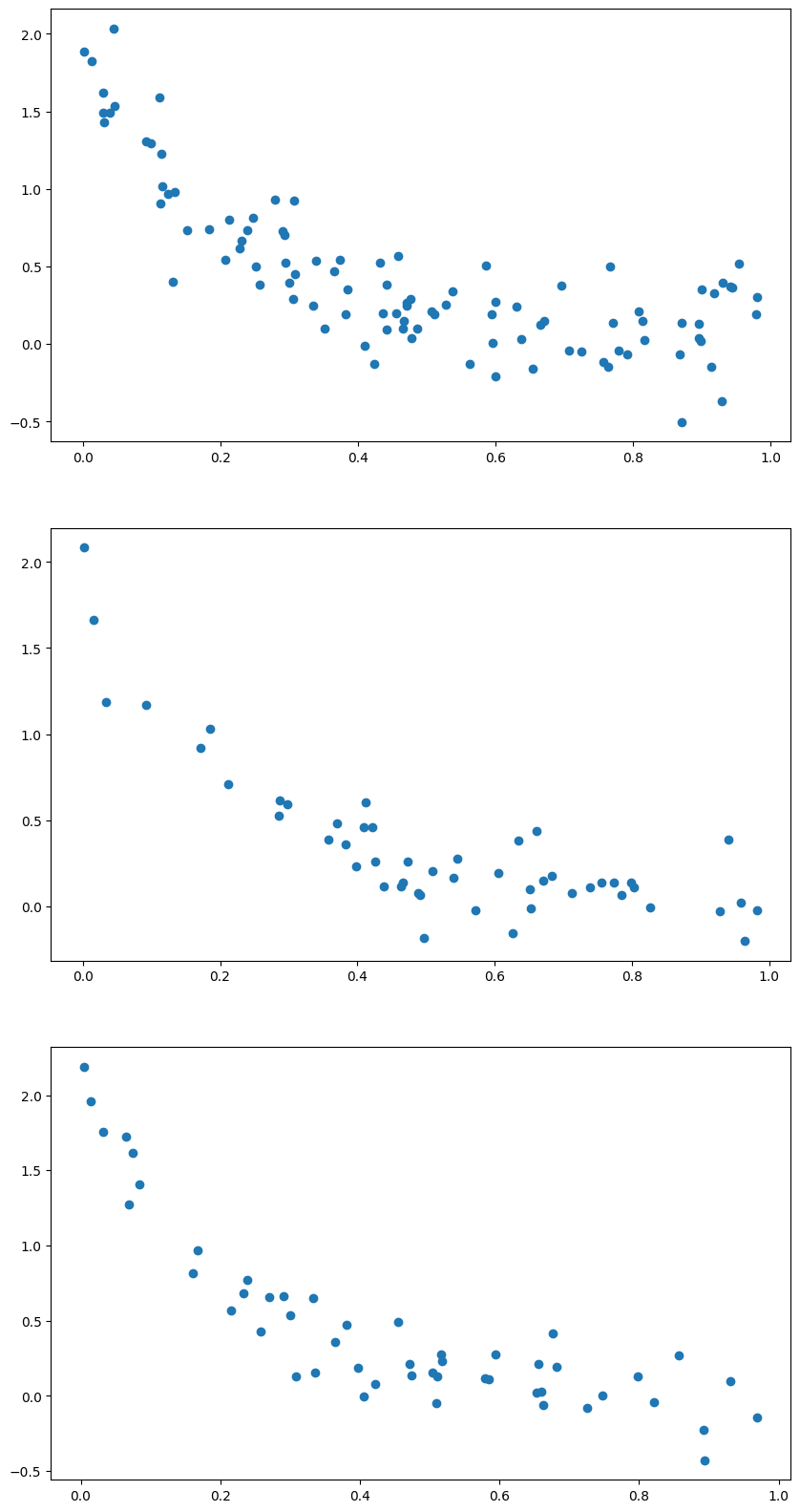
Before we start doing any analysis, we will separate the data at random into train, validate, and test sets. We will train our model (that is, find the weights \(w_i\)) on the first set, perform model comparison with the second set, and then test our selected model’s performance on the third set. Since it will have never seen the data from each set before, we can determine whether our model is performing well.

scikit-learn automatically comes with a function to do this, train_test_split, which we will import now. We will apply it twice to get our three sets:

from sklearn.model_selection import train_test_split

x_train, x_validate, y_train, y_validate = train_test_split(x, y, train_size = 0.5)
x_validate, x_test, y_validate, y_test = train_test_split(x_validate, y_validate, test_size = 0.5)

fig, ax = plt.subplots(1,3, figsize=(15,6))
ax[0].plot(x_train, y_train, 'o')
ax[1].plot(x_validate, y_validate, 'o')
ax[2].plot(x_test, y_test, 'o')

ax[0].set_title('Train')
ax[1].set_title('Validate')
ax[2].set_title('Test')

for i in range(3):
    ax[i].set_ylim(-1, 2)
    ax[i].set_xlabel('x')
    ax[i].set_ylabel('y')

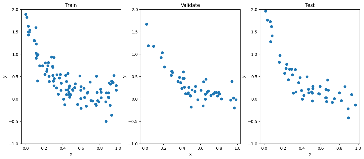
Notice that in the split we have done, the training set has twice as many data points in it as either the validate or the test sets. Generally, having more points in the training set will result in better performance of the model, but the specific split that is optimal is context-dependent.

Now, we’re performing a linear regression; again, we will use scikit-learn, which comes with a LinearRegression model in it. The fit method in that model requires a two-dimensional array of shape (samples, dimensions), so we will reshape our data to match its arguments:

#scikit-learn's linear regression model
from sklearn.linear_model import LinearRegression as LR


lr = LR()
lr.fit(x_train.reshape(-1, 1), y_train)

LinearRegression()

In a Jupyter environment, please rerun this cell to show the HTML representation or trust the notebook.
On GitHub, the HTML representation is unable to render, please try loading this page with nbviewer.org.

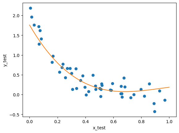
Now we can compare to our validate set to see how well the model works:

fig, ax = plt.subplots()
ax.plot(x_validate, y_validate, 'o')
ax.plot(x0.reshape(-1,1), lr.predict(x0.reshape(-1,1)), '-')
ax.set_ylabel('y')
ax.set_xlabel('x')
ax.set_ylim(-1,2)

(-1.0, 2.0)

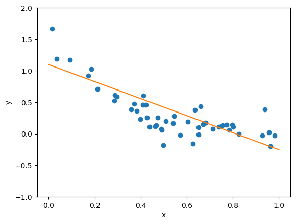
As we can see, our linear fit doesn’t really match the shape of the data particularly well. However, we only included two terms \(f(x) = w_0 \mathbb{1} + w_1 x\) in our fit, so we can always try truncating at higher order. We define a function to return the value of each basis function \(\phi_i\) for each data point \(x_j\) in the polynomial to \(n^{th}\) order. What this means is that at first order, this function will return an Nx1 array, which contains all the \(x_i\) values from \(i = 1\) to \(i = N\). At second order, it will return an Nx2 array, where the first column is all the values \(x_i\) and the second column is all the values \(x_i^2\); at third order we will have a third column with the values \(x_i^3\), and so forth.

def nth_polynomial(x, n):
    return np.stack([x**i for i in range(1, n+1)], axis=1)

Now we will try fitting our data to the polynomial at successively higher orders. It is important to note that when we ask for a linear regression, we are handing the LinearRegression().fit object a series of values. Recall that the linear regression in general has \(f(x_i) = \sum_j(w_j \phi_j)\). When we are training a model (asking for a fit), we are handing the model an arbitrary number of \(\phi_j\) and asking it to compute the coefficients \(w_j\); that is, we must compute the values of the basis functions for each data point ourselves. For example, suppose we were interested in fitting to a cubic polynomial, so that the fit is to the model \(f(x_i) = w_0 + w_1 x_i + w_2 x_i^2 + w_3 x_i^3\). The information we hand the LinearRegression().fit function is the value of \(x_i\), \(x_i^2\), and \(x_i^3\). If instead, we were interested in fitting to a Fourier series, we would need to hand the function the values of \(e^{2\pi i x}, \)e^{4\pi i x}\(, \)e^{6\pi i x}$, and so forth.

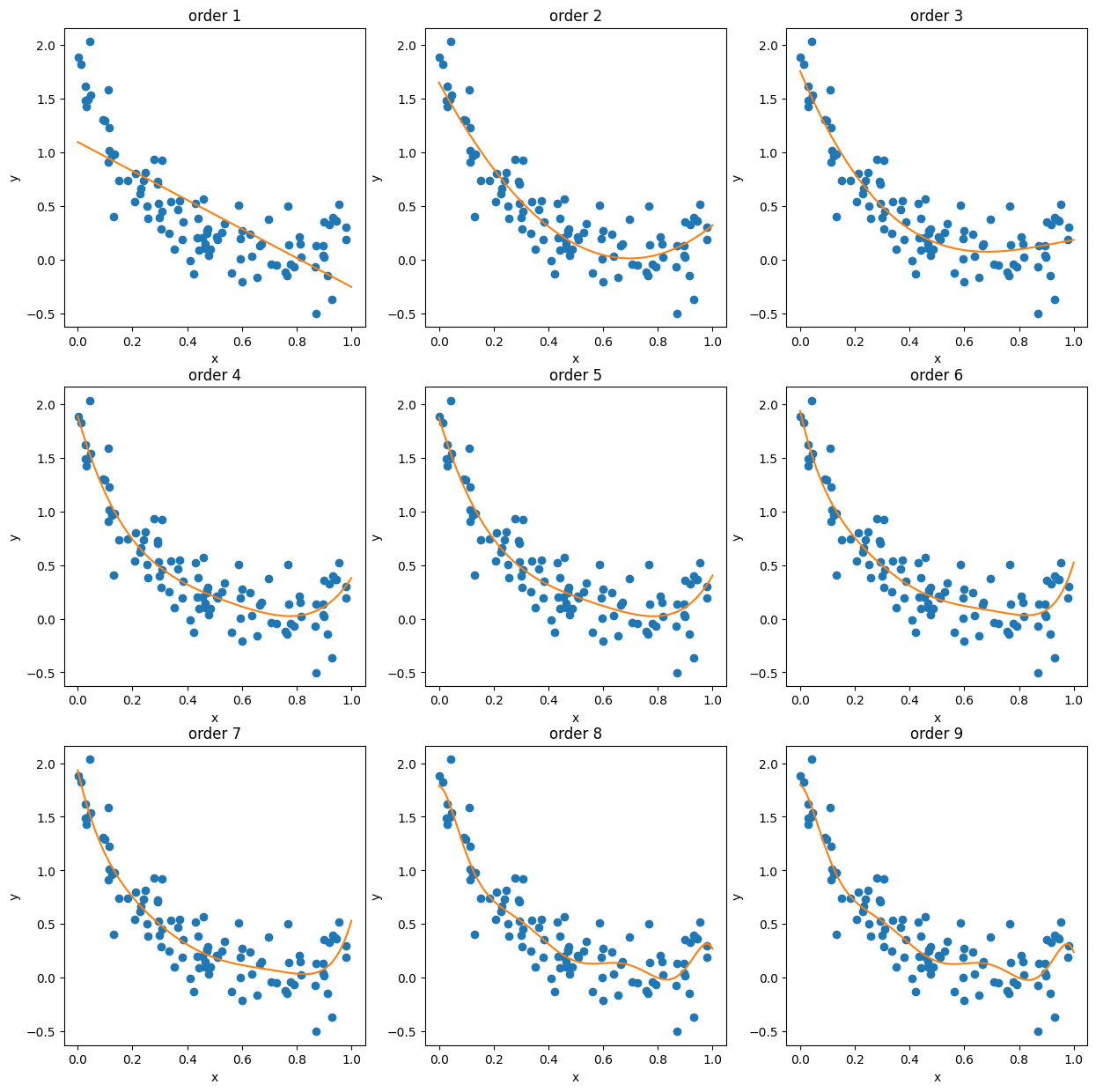
Now we’ll compare the fits to the training data:

max_order = 9

lr_list = [LR() for i in range(max_order)]
for i, lr in enumerate(lr_list):
    x_nth = nth_polynomial(x_train, i+1)
    lr.fit(x_nth, y_train)
    
fig, ax = plt.subplots(3,3, figsize=(15,15))

for i, lr in enumerate(lr_list):
    xi = i%3
    yi = i//3
    x_nth = nth_polynomial(x0, i+1)
    ax[yi, xi].plot(x_train, y_train, 'o')
    ax[yi, xi].plot(x0, lr.predict(x_nth))
    ax[yi, xi].set_xlabel('x')
    ax[yi, xi].set_ylabel('y')
    ax[yi, xi].set_title('order '+str(i+1))

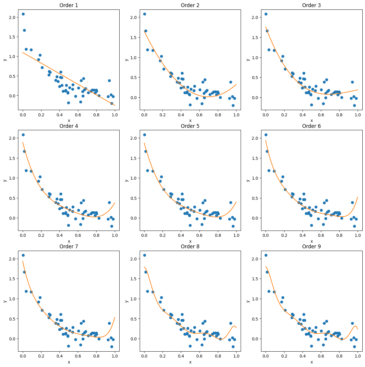
And now we can compare them to the validation set:

fig, ax = plt.subplots(3,3, figsize=(15,15))

for i, lr in enumerate(lr_list):
    xi = i%3
    yi = i//3
    x_nth = nth_polynomial(x0, i+1)
    ax[yi, xi].plot(x_validate, y_validate, 'o')
    ax[yi, xi].plot(x0, lr.predict(x_nth))
    ax[yi, xi].set_xlabel('x')
    ax[yi, xi].set_ylabel('y')
    ax[yi, xi].set_title('Order '+str(i+1))

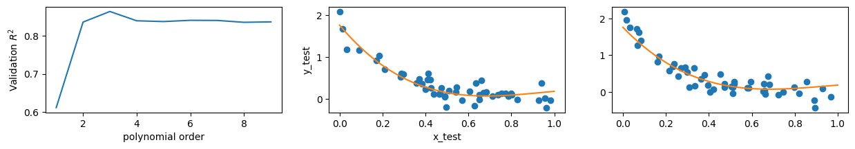
Since comparing by eye is imprecise, it would be better to see how the fits perform quantitatively. Since we’re testing the model’s validity, we’ll use the \(R^2\) value to gauge their goodness-of-fit here - the coefficient of determination measures how much of the target’s variance is explained by the model, which is precisely what we want. (Contrast this, for example, with the \(\chi^2\) measure, which measures how much the target depends on a particular feature.) We will try to maximize our \(R^2\) value and we will compare it to our test set:

R2_vals = []

for i, lr in enumerate(lr_list):
    x_nth = nth_polynomial(x_validate, i+1)
    R2 = lr.score(x_nth, y_validate)
    R2_vals.append(R2)

order = np.arange(1,max_order+1)
fig, ax = plt.subplots(1,3, figsize=(15,2))
ax[0].plot(order, R2_vals)
ax[0].set_ylabel('Validation $R^2$')
ax[0].set_xlabel('polynomial order')

best_model_index = np.argmax(R2_vals)
lr_best = lr_list[best_model_index]

ax[1].plot(x_validate, y_validate, 'o')
x_nth = nth_polynomial(x0, best_model_index+1)
ax[1].plot(x0, lr_best.predict(x_nth))
ax[1].set_ylabel('y_validate')
ax[1].set_xlabel('x_validate')


ax[2].plot(x_test, y_test, 'o')
ax[2].plot(x0, lr_best.predict(x_nth))
ax[1].set_ylabel('y_test')
ax[1].set_xlabel('x_test')

print("Best model is order:  {}".format(best_model_index+1))

Best model is order:  5

One thing we must be aware of as we increase the order of our fits is the possibility of overfitting. As we add more features to our model and ask it to approximate the data, it will perform better and better specific to the data it is being trained on. This does not mean it is performing better in general! Overfitting occurs when the model becomes hyperspecific to the data it was trained on. As an example, one could imagine training an AI to identify hands, by presenting it with images of people with their fingers outstretched. If those are the only images it’s trained on the AI may decide that the defining feature of a hand is the presence of five fingers, and stop identifying hands in pictures of people with their fingers closed.

Thus, there is a precise tuning that we must do with these kinds of models. If we include too few features, we may end up underfitting and our model will have no predictive power. If we include too many features, we may overfit and our model will likewise have no predictive power.

More Ways to do Cross-Validation

The process we have done above is called cross-validation. We did it by hand, but there are multiple tools to quickly cross-validate a model. Here, we will see two other methods using scikit-learn and two of its functions cross_validate and KFold.

The motivation for using k-folds is as follows. Validating a model only once is like running an experiment only once; we cannot be sure of our results, but we can increase our certainty by repeating the experiment, or in the case of regression, by performing multiple validations. k-fold cross-validation is designed to do this. In it, the data is split into \(k\) sets (called folds), where the value of \(k\) is a free parameter for you to choose, and each set is labeled by its number. The model is then trained on the data modulo the first fold and cross-validation is done using the first fold as a test set. The weights are then reset and the model is trained on all the data modulo the second fold; cross validation is then done using the second fold as a test set. This is repeated until every fold has been used to test the data, and \(k\) trained models have been generated. The performance of all the models is then averaged to determine the overall performance of that particular model.

The cross_validate function natively uses a k-fold process when it performs cross-validation. We demonstrate the use of these functions below.

For simplicity, we will reuse our dataset from above and compare our various models’ performances. The cross_validate function’s arguments here are (object to use for fit, data to fit, target data, cv = number of folds). The object to use for fit in this case is the LR(), instructing the function to use a linear regression. We provide the values of the basis functions \(\phi_i\) for each order as the data to fit to in the second argument. The third argument are the target values, i.e. the corresponding \(y\) values to each \(x_i\). The fourth argument is the number of folds to use for the k-fold process.

from sklearn.model_selection import cross_validate

cv_mean_error = np.zeros_like(lr_list)

for i, lr in enumerate(lr_list):
    x_nth = nth_polynomial(x_train, i+1)
    cv_dict = cross_validate(lr, x_nth, y_train, cv=4)
    cv_mean_error[i] = np.mean(cv_dict['test_score'])
    
print(cv_mean_error)
fig, ax = plt.subplots()
ax.plot(cv_mean_error)
ax.set_ylabel('Cross Validation $<R^2>$')
ax.set_xlabel('polynomial order')

[0.6615985156765863 0.8046321835062282 0.820135931754942
 0.8165462043796976 0.8271219647654617 0.8237127979082467
 0.8146713275793759 0.8097969839544833 0.8145440456227531]

Text(0.5, 0, 'polynomial order')

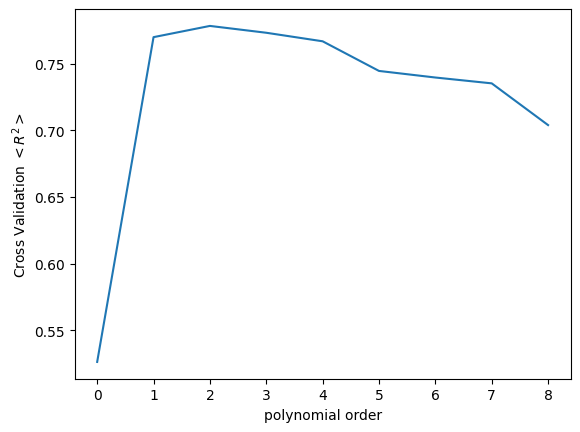
The output of the cross_validate function is a Dictionary type object, with a variety of keys that can be used to access details about the cross-validation. Here, we are mainly interested in the 'test_score' key, and we average over the results from all the k-folds in order to assess the performance of the model.

Or we can also use KFold directly.

from sklearn.model_selection import KFold

va, (ax1, ax2, ax3) = plt.subplots(3,1, figsize = (10,20))
ax1.plot(x_train, y_train, 'o')
ax2.plot(x_validate, y_validate, 'o')
ax3.plot(x_test, y_test, 'o')

[<matplotlib.lines.Line2D at 0x7fdfbde96ec0>]

folds = KFold(n_splits=4)

scores = np.zeros_like(lr_list)

for i, lr in enumerate(lr_list):
    scores_temp = []
    for train, test in folds.split(x_train):
        x_nth = nth_polynomial(x_train[train], i+1)
        lr.fit(x_nth, y_train[train])
        x_nth = nth_polynomial(x_train[test], i+1)
        scores_temp.append(lr.score(x_nth, y_train[test]))
    scores[i] = np.mean(scores_temp)
        

fig, ax = plt.subplots()
ax.plot(scores)
ax.set_ylabel('Cross Validation $<R^2>$')
ax.set_xlabel('polynomial order')
# ax.set_ylim(-0.25, 0.25)

Text(0.5, 0, 'polynomial order')

Regardless of which method we choose, the cross-validation process will give us a best fit model. Finally, we can apply that model we find to the test data:

best_model_index = np.argmax(scores)
lr_best = lr_list[best_model_index]
x_nth = nth_polynomial(x_train, best_model_index+1)
lr_best.fit(x_nth, y_train)

fig, ax = plt.subplots()
ax.plot(x_test, y_test, 'o')
x_nth = nth_polynomial(x0, best_model_index+1)
ax.plot(x0, lr_best.predict(x_nth))
ax.set_ylabel('y_test')
ax.set_xlabel('x_test')

Text(0.5, 0, 'x_test')

As we can see here, our model roughly matches the shape of the data; it’s not perfect, but it does seem to have relatively good predictive power; it doesn’t exactly match the data, but it’s relatively close.

Other methods of regression do exist to try to improve on this. One extension, for example, is the generalized linear model, which permits us to add a degree of non-linearity to our regression (this is the topic of another tutorial). The method of fitting you should select should ultimately be specific to the experiment and features of the data you are interested in, as different models will perform better or worse in different circumstances.

Regression on a real data set

Next, we’ll move on to doing regression on a real life dataset. We’ll use data from the Allen Brain Observatory’s Visual Coding dataset to do this, to study neural activity based on animal running speed. First, we’ll need to actually access the dataset using the AllenSDK.

The following block of code accesses the Visual Coding 2-Photon dataset from the ABO, and then pulls data from an example experiment.

from allensdk.core.brain_observatory_cache import BrainObservatoryCache

manifest_path = "/data/allen-brain-observatory/visual-coding-2p/manifest.json"
boc = BrainObservatoryCache(manifest_file = manifest_path)

import pandas as pd

expt_container_id = 637998953
cell_id = 662191687

expt_session_info = boc.get_ophys_experiments(experiment_container_ids = [expt_container_id])
expt_session_info_df = pd.DataFrame(expt_session_info)

session_id = expt_session_info_df[expt_session_info_df.session_type=='three_session_A'].id.iloc[0]
data_set = boc.get_ophys_experiment_data(ophys_experiment_id = session_id)

cell_idx = data_set.get_cell_specimen_indices([cell_id])[0]
events = boc.get_ophys_experiment_events(ophys_experiment_id = session_id)
events_time = data_set.get_fluorescence_timestamps()

dx, dx_time = data_set.get_running_speed()

We’ll start by simply examining the raw data. The two variables we’re interested in examining are running speed and df/f trace. Let’s show the raw data, filtered to ignore any extraneous outliers:

from scipy import signal

dx_filtered = signal.medfilt(dx,3)

fig, (ax1,ax2) = plt.subplots(2,1,figsize=(8,8))
ax1.plot(events_time, events[cell_idx,:], 'b')
ax1.set_xlabel("Time (s)")
ax1.set_ylabel("dF/f")

ax2.plot(dx_time, dx_filtered, 'k')
ax2.set_xlabel("Time (s)")
ax2.set_ylabel("Running speed (cm/s)")
plt.show()

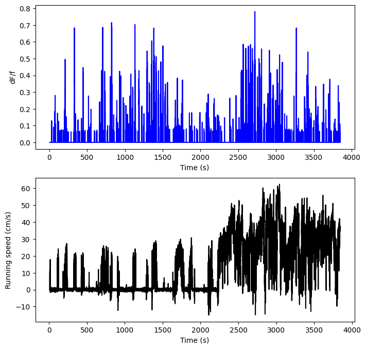
It’s certainly hard to tell, but it looks like there might be a connection here. Both of these are plotted against time, and they both have a lot of change over the course of the experiment, but it’s hard to tell if they occur around the same times, or if there’s a relationship of some kind between dff and running speed. A regression might help. As above, we start by splitting our data.

print(dx_filtered)

print(len(dx_filtered))
print(len(events))

[nan nan nan ... nan nan nan]
115469
99

L = dx.shape[0]

dx_train = dx[:L//2]
dx_validate = dx[L//2:3*L//4]
dx_test = dx[3*L//4:]

events_train = events[:,:L//2]
events_validate = events[:,L//2:3*L//4]
events_test = events[:,3*L//4:]

For this particular regression, we’ll also bin our data, so that we can group data points that are roughly similar to each other. We’ll lose some granularity and predictive power, but we’ll make the analysis faster and simpler.

def binning(a, bin_edges, alt_array=None):
    n = len(bin_edges)-1
    a_binned = np.zeros(n)
    if alt_array is not None:
        alt_binned_list = [np.zeros(n) for t in alt_array]
    for i in range(n):
        lower = bin_edges[i]
        upper = bin_edges[i+1]
        bin_mask = np.logical_and(a >= lower, a < upper)
        a_masked = a[bin_mask]
        if len(a_masked)>0:
            a_binned[i] = np.mean(a_masked)
        else:
            a_binned[i] = 0
        if alt_array is not None:
            for j in range(len(alt_array)):
                vals = alt_array[j][bin_mask]
                if len(vals)>0:
                    alt_binned_list[j][i] = np.mean(vals)
                else:
                    alt_binned_list[j][i] = 0
        
    if alt_array is not None:
        return a_binned, alt_binned_list
    else:
        return a_binned
    
bin_edges = np.linspace(0,40,100)

running_bin_train, events_bin_train = binning(dx_train, bin_edges, [events_train[cell_idx]])
running_bin_validate, events_bin_validate = binning(dx_validate, bin_edges, [events_validate[cell_idx]])
running_bin_test, events_bin_test = binning(dx_test, bin_edges, [events_test[cell_idx]])

events_bin_train = events_bin_train[0]
events_bin_validate = events_bin_validate[0]
events_bin_test = events_bin_test[0]

And now we can do the regression. We’ll do it to several orders, like above, so we can compare several different models.

max_order = 9

lr_list = [LR() for i in range(max_order)]
for i, lr in enumerate(lr_list):
    running_nth_order = nth_polynomial(running_bin_train, i+1)
    lr.fit(running_nth_order, events_bin_train)

fig, ax = plt.subplots(3,3, figsize=(15,15))

for i, lr in enumerate(lr_list):
    xi = i%3
    yi = i//3
    running_nth_order = nth_polynomial(running_bin_train, i+1)
    ax[yi, xi].plot(running_bin_train, events_bin_train, 'o')
    ax[yi, xi].plot(running_bin_train, lr.predict(running_nth_order),'o')
    ax[yi, xi].set_xlabel('Running Speed (cm/s)')
    ax[yi, xi].set_ylabel('Response (dF/f)')
    ax[yi, xi].set_title('Order '+str(i+1))

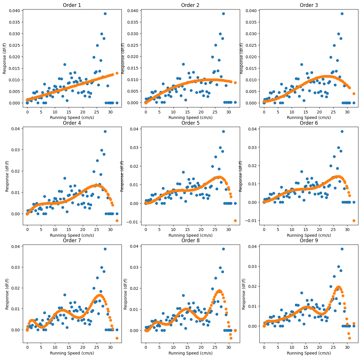
But as ever, we also need to check how these perform on data they’ve never seen before. Enter the validation sets:

fig, ax = plt.subplots(3,3, figsize=(15,15))

for i, lr in enumerate(lr_list):
    xi = i%3
    yi = i//3
    ax[yi, xi].plot(running_bin_validate, events_bin_validate, 'o')
    running_nth_order = nth_polynomial(running_bin_validate, i+1)
    ax[yi, xi].plot(running_bin_validate, lr.predict(running_nth_order),'o')
    ax[yi, xi].set_xlabel('Running Speed (cm/s)')
    ax[yi, xi].set_ylabel('Response (dF/f)')
    ax[yi, xi].set_title('Order '+str(i+1))

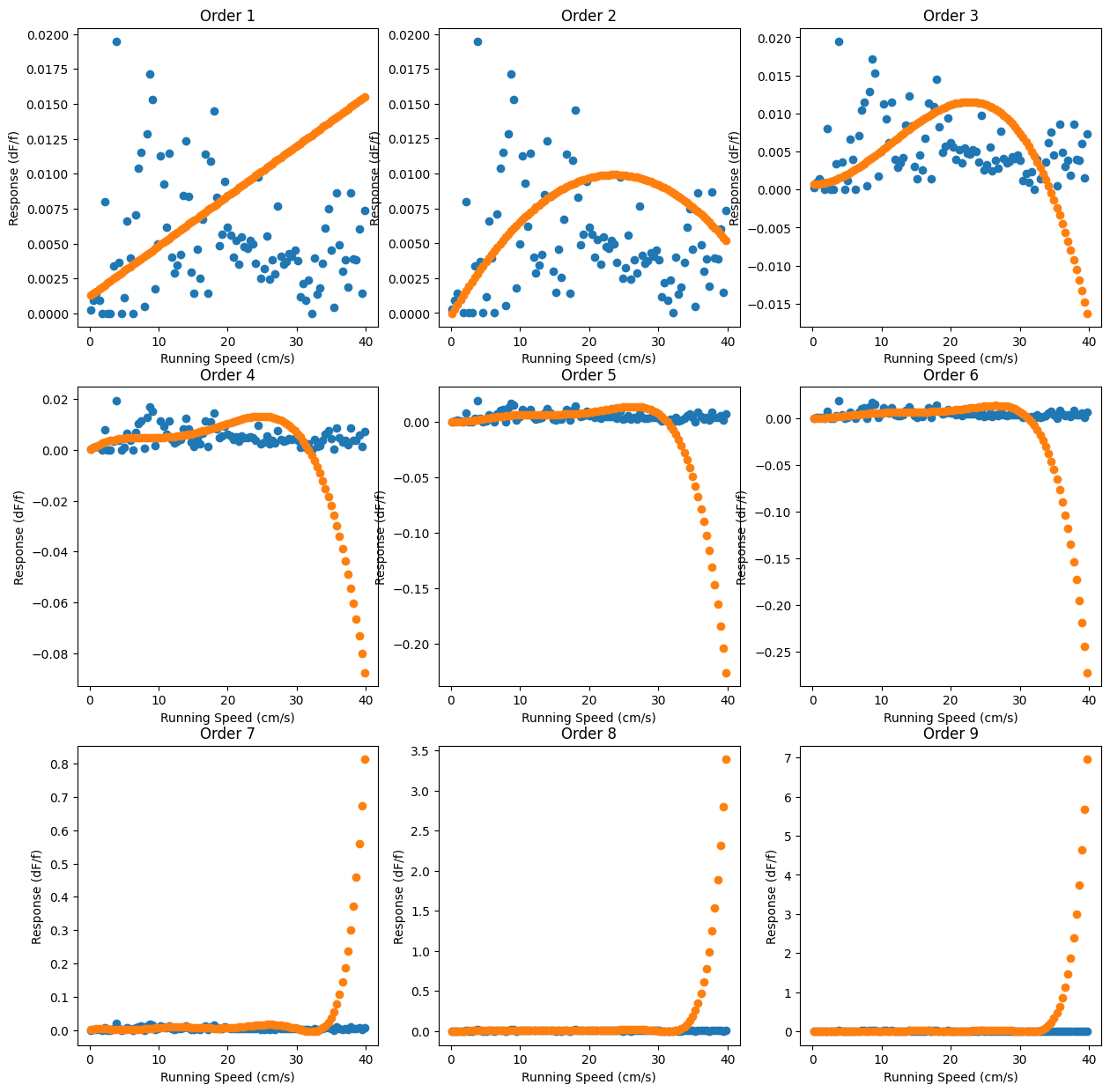
Yikes! These don’t look much like the validation data at all. Nevertheless, the eye isn’t a good way to gauge things, so we’ll compute their scores to evaluate their performance numerically:

R2_vals = []

for i, lr in enumerate(lr_list):
    running_nth_order = nth_polynomial(running_bin_validate, i+1)
    R2 = lr.score(running_nth_order, events_bin_validate)
    R2_vals.append(R2)
    
order = np.arange(1,len(R2_vals)+1)

best_model_index = np.argmax(R2_vals)
lr_best = lr_list[best_model_index]

running_nth_order = nth_polynomial(running_bin_train, best_model_index+1)
print(lr_best.score(running_nth_order, events_bin_train))

0.33187918902886937

So once we use data the models haven’t seen before, we find that around 30% of the variance in our data is explained by this model. There’s certainly other factors confounding this analysis, but at the least, it seems like there’s some correlation between the running speed and the df/f.

To summarize regression: we are supposing that some linear combination of functions will provide a decent approximation of the relationship in our data (this is called choosing the model). We then apply the functions and variationally calculate the relevant coefficients by attempting to minimize an error function that we establish (this is called training the model). Finally, we compare the models that we’ve generated to holdout data that it has not seen before and examine how they perform (validating the model).